异常值分析方法

3σ 原则(数据接近正态分布时使用)与箱线图分析法

---

箱线图

1. 箱线图异常值分析

QL：下四分位数

QU：上四分位数

IQR：QU - QL，上四分位数与下四分位数之差

whis：权重

异常值为：< QL - whis * IQR 以及 > QU + whis * IQR 部分

2. 箱线图绘制 plt.boxplot

import matplotlib.pyplot as plt

p = plt.boxplot(序列, notch=True, whis=1.5, labels=标签列表)
# 序列可以是多个数组组成的列表，每个数组对应一个箱体，一次对应标签列表中的标签
# 只考察画一个箱体的图，如下
p = plt.boxplot(序列, notch=True, whis=1.5, labels=['箱体的标签'])
# 序列是画图的数据，一维
# notch是箱体凹口，50%分位标记
# whis是，上下超过IQR*whis的标记为异常点
# labels中只放一个字符串作为这个箱体的标签

3. 箱线图绘制后提取异常值

import matplotlib.pyplot as plt

# 画箱线图，并且返回对象给p
p = plt.boxplot(df['data'], notch=True, whis=1.5, labels=['标签'])

# p对象中，fliers放异常值
# 因为只画了一个箱体，也就是第一个箱体，所以是索引0
# .get_ydata()方法获取y坐标，为实际的数据的值
outlier1 = p['fliers'][0].get_ydata()

# 输出异常值的值
print('异常值为：', outlier1)

# 输出df中data异常行，每行的索引即为异常值的索引（如需单独给出索引的话）
print(df[df['data'].isin(outlier1)])

---

练习题1

创建一个有50个元素的Series对象，其values数组中的数据随机生成，数据总体上满足均值为1000, 标准差为200的正态分布。

(1) 自定义异常值为：小于QL-1.25IQR或大于QU+1.25IQR的值。绘制箱线图，检测生成的数据中是否包含大于上限和小于下限的异常值，并且要求这两类异常值都要有。如果不满足要求，那么就重新生成数据，直到满足要求为止；

(2) 利用箱线图获取并输出异常值的索引；

(3) 编写一个通用函数，其功能为将一个Series对象中大于上限的异常值用QU替换，而小于下限的异常值用QL替换。（在该函数中设置一个inplace=False的默认值参数，如果实参传过来的值为True，则表示修改会在Series对象中保留）

(4) 用该函数处理满足(1)要求的Series对象，输出QU、QL的值。然后，创建一个如下所示的DataFrame对象，其index为异常值的索引，Before列上的数据为替换前的值，After列上的数据为替换后的值。最后，输出该DataFrame对象。

测试时一次非原地操作，一次原地操作

输出示例：

QU = 1153.800, QL= 897.075

       Before   After

31   518.7     897.075

32   1525.1   1153.800

38   495.0     897.075

47   1657.5   1153.800

# 本人思路，仅供参考
import numpy as np
import pandas as pd
import matplotlib.pyplot as plt

# (1)
values1 = np.random.normal(1000, 200, size=50)
ser1 = pd.Series(values1)
print(ser1)

# (2)
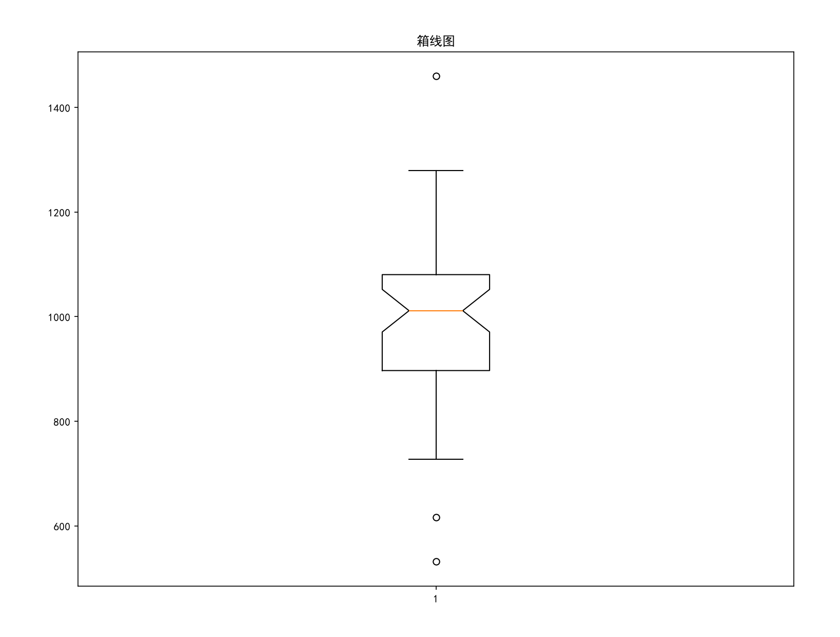
plt.figure(figsize=(12, 9))
plt.title('箱线图')
whiss = 1.25
p = plt.boxplot(ser1, notch=True, whis=whiss)
plt.show()
outliers1 = p['fliers'][0].get_ydata()
indexx = list(ser1[ser1.isin(outliers1)].index)
print(indexx)


# (3)
def func(ser, inplace=False):
    qu, ql = np.quantile(ser, [0.25, 0.75])
    iqr = qu - ql
    if inplace:
        ser[ser > qu + whiss * iqr] = qu
        ser[ser < ql - whiss * iqr] = ql
        ser1 = ser
    else:
        ser1 = ser.copy()
        ser1[ser1 > qu + whiss * iqr] = qu
        ser1[ser1 < ql - whiss * iqr] = ql
    return ql, qu, ser1


# (4)
ser0 = ser1.copy()
ql2, qu2, ser2 = func(ser1)
ql3, qu3, ser3 = func(ser1, inplace=True)

before = ser0.iloc[indexx]
after2 = ser2.iloc[indexx]
after3 = ser3.iloc[indexx]

df2 = pd.DataFrame({'Before': before, 'After': after2}, index=indexx)
df3 = pd.DataFrame({'Before': before, 'After': after3}, index=indexx)

print(f'QU = {qu2}, QL = {ql2}')
print(df2)

print(f'QU = {qu3}, QL = {ql3}')
print(df3)

---

标准化方法

1. 最小-最大标准化

公式：

2. 标准差标准化

公式：

3. 小数定标标准化

公式：

其中 k 和数据中绝对值最大的数的整数位数有关，非 10 的幂则为这个数的整数位数，10 的幂次方则为整数位数 -1：

例如：

绝对值最大的数为999，则k=3；绝对值最大的数为1000，则k=3；绝对值最大的数为1001，则k=4

import numpy as np

k = np.ceil(np.log10(data.abs().max()))
data = data / 10 ** k

---

练习题2

读取通过第九章(上)练习题1(包含在资源绑定中)获得的“Scores.xlsx”文件中的数据。编写3个通用函数，分别实现最小-最大标准化、标准差标准化（处理后数据的均值和标准差算出来打印）和小数定标标准化的功能。然后，按最小-最大标准化处理“C++”成绩列上的数据，按标准差标准化处理“Java”成绩列上的数据，按小数定标标准化处理“Python”成绩列上的数据。最后，输出处理后的结果。

# 本人思路，仅供参考
import numpy as np
import pandas as pd

scores = pd.read_excel('./Scores.xlsx')
print(scores)

def maxmin(ser):
    ser = (ser - ser.min()) / (ser.max() - ser.min())
    return ser

def stdd(ser):
    ser = (ser - ser.mean()) / ser.std()
    ave = ser.mean()
    stdd = ser.std()
    print(f'处理后均值：{ave} 处理后方差：{stdd}')
    return ser

def lit(ser):
    k = np.ceil(np.log10(ser.abs().max()))
    ser = ser / 10 ** k
    return ser
    
print(maxmin(scores['C++']))
print(stdd(scores['Java']))
print(lit(scores['Python']))

---

数据离散化/分箱

1. 等宽法

import pandas as pd

# 等宽法分箱
cut1 = pd.cut(数组/Series, 整数/序列, right=True, include_lowest=False)
# 第二个参数若为整数表示分箱个数（等宽等分），若为序列则按序列每两个数分一个区间，数表示区间边界
# right为True左开右闭，为False左闭右开
# include_lowest为True会让最左边区间端点变得更小一点，把最小值包含进去

# 输出分箱结果
print(cut1)

# 查看各分箱区间元素数
print(cut1.value_counts())

# 分箱区间改名
cut1.rename_categories(字符串序列)
或
cut1.cat.rename_categories(字符串序列)

传入数组、列表时，cut 会返回 categorical 对象，可以直接使用 rename_categories 方法进行分箱区间改名；

传入 Series 时，cut 会返回 Series 对象，必须先使用 .cat 方法再用 rename_categories 方法才能进行分箱区间改名。

import numpy as np
import pandas as pd

lst1 = [2, 65, 13, 2, 31, 5, 6, 89]
arr1 = np.array(lst1)
ser1 = pd.Series(lst1)


cut1 = pd.cut(ser1, [0, 25, 50, 100], right=True, include_lowest=False)
cut2 = pd.cut(arr1, [0, 25, 50, 100], right=True, include_lowest=False)
cut3 = pd.cut(lst1, [0, 25, 50, 100], right=True, include_lowest=False)

# 分箱区间改名
cut1 = cut1.cat.rename_categories(['区间一', '区间二', '区间三'])
print(cut1)
'''
0    区间一
1    区间三
2    区间一
3    区间一
4    区间二
5    区间一
6    区间一
7    区间三
dtype: category
Categories (3, str): ['区间一' < '区间二' < '区间三']
'''

cut2 = cut2.rename_categories(['区间一', '区间二', '区间三'])
print(cut2)
'''
['区间一', '区间三', '区间一', '区间一', '区间二', '区间一', '区间一', '区间三']
Categories (3, str): ['区间一' < '区间二' < '区间三']
'''

cut3 = cut3.rename_categories(['区间一', '区间二', '区间三'])
print(cut3)
'''
['区间一', '区间三', '区间一', '区间一', '区间二', '区间一', '区间一', '区间三']
Categories (3, str): ['区间一' < '区间二' < '区间三']
'''

例题：

对ser1 = pd.Series([2, 65, 13, 2, 31, 5, 6, 89])分箱为4个区间，查看各分箱区间元素数，查看分箱区间，将区间名改为['区间一', '区间二', '区间三', '区间四']后再次查看分箱区间，查看各分箱区间元素数，查看各分箱区间元素数，查看每个数据点对应的分组

import pandas as pd

lst1 = [2, 65, 13, 2, 31, 5, 6, 89]
ser1 = pd.Series(lst1)

# 分箱
cut1 = pd.cut(ser1, 4, right=True, include_lowest=False)

# 查看各分箱区间元素数
print(cut1.value_counts())
'''
(1.913, 23.75]    5
(23.75, 45.5]     1
(45.5, 67.25]     1
(67.25, 89.0]     1
Name: count, dtype: int64
'''

# 查看分箱区间
print(cut1.cat.categories)
'''
IntervalIndex([(1.913, 23.75], (23.75, 45.5], (45.5, 67.25], (67.25, 89.0]], dtype='interval[float64, right]')
'''

# 分箱区间改名
cut1 = cut1.cat.rename_categories(['区间一', '区间二', '区间三', '区间四'])

# 查看分箱区间
print(cut1.cat.categories)
'''
Index(['区间一', '区间二', '区间三', '区间四'], dtype='str')
'''

# 查看各分箱区间元素数
print(cut1.value_counts())
'''
区间一    5
区间二    1
区间三    1
区间四    1
Name: count, dtype: int64
'''

# 按顺序查看每个数据点对应的分组
print(cut1.values)
'''
['区间一', '区间三', '区间一', '区间一', '区间二', '区间一', '区间一', '区间四']
Categories (4, str): ['区间一' < '区间二' < '区间三' < '区间四']
'''

2. 等频法

import pandas as pd

# 等频法分箱
qcut1 = pd.qcut(数组/Series, 整数/分位数序列)
# 第二个参数为整数，则分为整数份，每份频率大体相等
# 若第二个参数为序列，则里面值必须为0~1之间的数，表示分位点的位置。序列必须严格递增

# 查看区间边界
print(f'区间边界：{qcut1.categories}')    # .categories为属性，并非函数，不用带括号

---

练习题3

随机生成20个[40, 100)之间的成绩，分别按下面的要求离散化。

(1) 指定区间边界为[0, 60, 70, 80, 90, 100]，输出分箱结果（左闭右开）并统计各区间数据的个数，然后，依次把各区间的标签改为E、D、C、B、A，再次查看各区间数据的个数。

(2) 使用等宽法离散化数据，5个区间。输出分箱结果并统计各区间数据的个数。

(3) 使用等频法离散化数据，5个区间。要求先使用quantile函数计算分位数，然后用cut函数完成分箱，最后输出分箱后的区间名并统计各区间数据的个数。

(4) 使用等频法离散化数据，5个区间。要求用qcut函数实现，查看和(3)的结果是否一致。

# 本人思路，仅供参考
import numpy as np
import pandas as pd

scores = np.random.randint(40, 100, 20)    # 注意randint函数的区间边界是左闭右开
print(scores)

# (1)
b = [0, 60, 70, 80, 90, 100]
cut1 = pd.cut(scores, b, right=False)
# 输出分箱结果
print(cut1)
# 统计元素个数
print(cut1.value_counts())

# 改标签
cut1 = cut1.rename_categories(['E', 'D', 'C', 'B', 'A'])
# 再输出分箱结果
print(cut1)
# 再统计元素个数
print(cut1.value_counts())

# (2)
cut2 = pd.cut(scores, 5)
print(cut2)
print(cut2.value_counts())

# (3)
q = [0, 0.2, 0.4, 0.6, 0.8, 1.0]
# 计算分位数
qns = np.quantile(scores, q)
qcut1 = pd.cut(scores, qns, include_lowest=True)
print(qcut1)
print(f'区间边界：{qcut1.categories}')
print(qcut1.value_counts())

# (4)
qcut2 = pd.qcut(scores, 5)
print(qcut2)
print(f'区间边界：{qcut2.categories}')
print(qcut2.value_counts())