机器学习-第三章 线性回归 下
·
机器学习-第三章 线性回归 下
3. 线性回归模型评估
1.为什么要进行模型评估
衡量预测值和真实值之间的差距
2.误差种类
MSE 均方误差
MAE 平均绝对误差
RMSE 均方根误差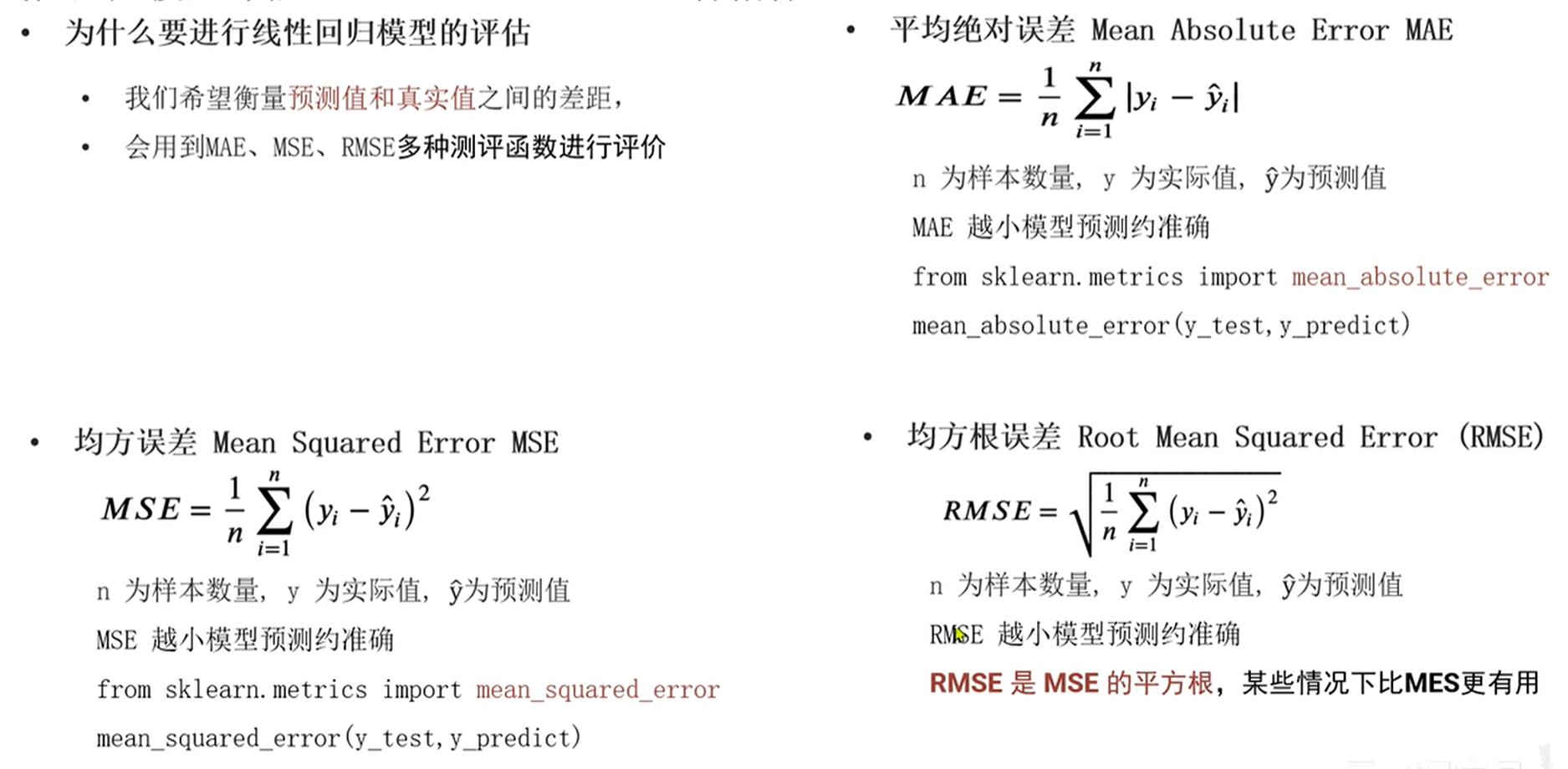
3.指标对比
MSE 均方误差
MAE 平均绝对误差
RMSE 均方根误差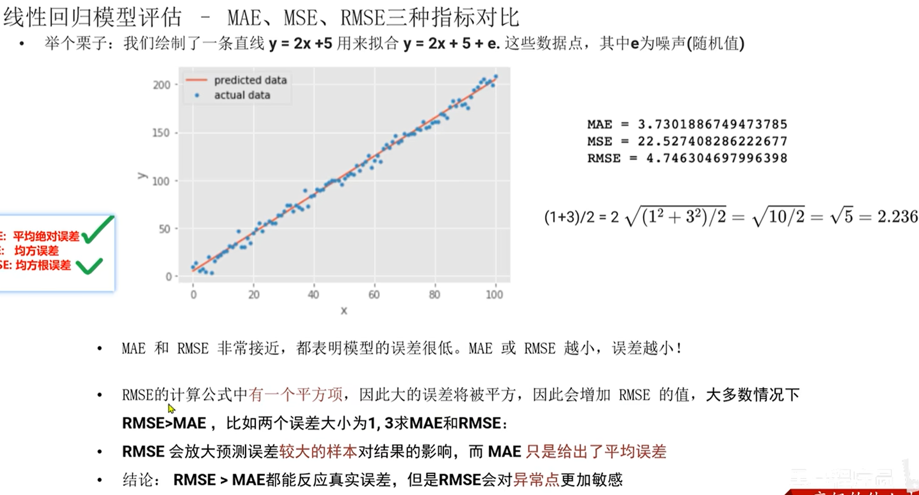
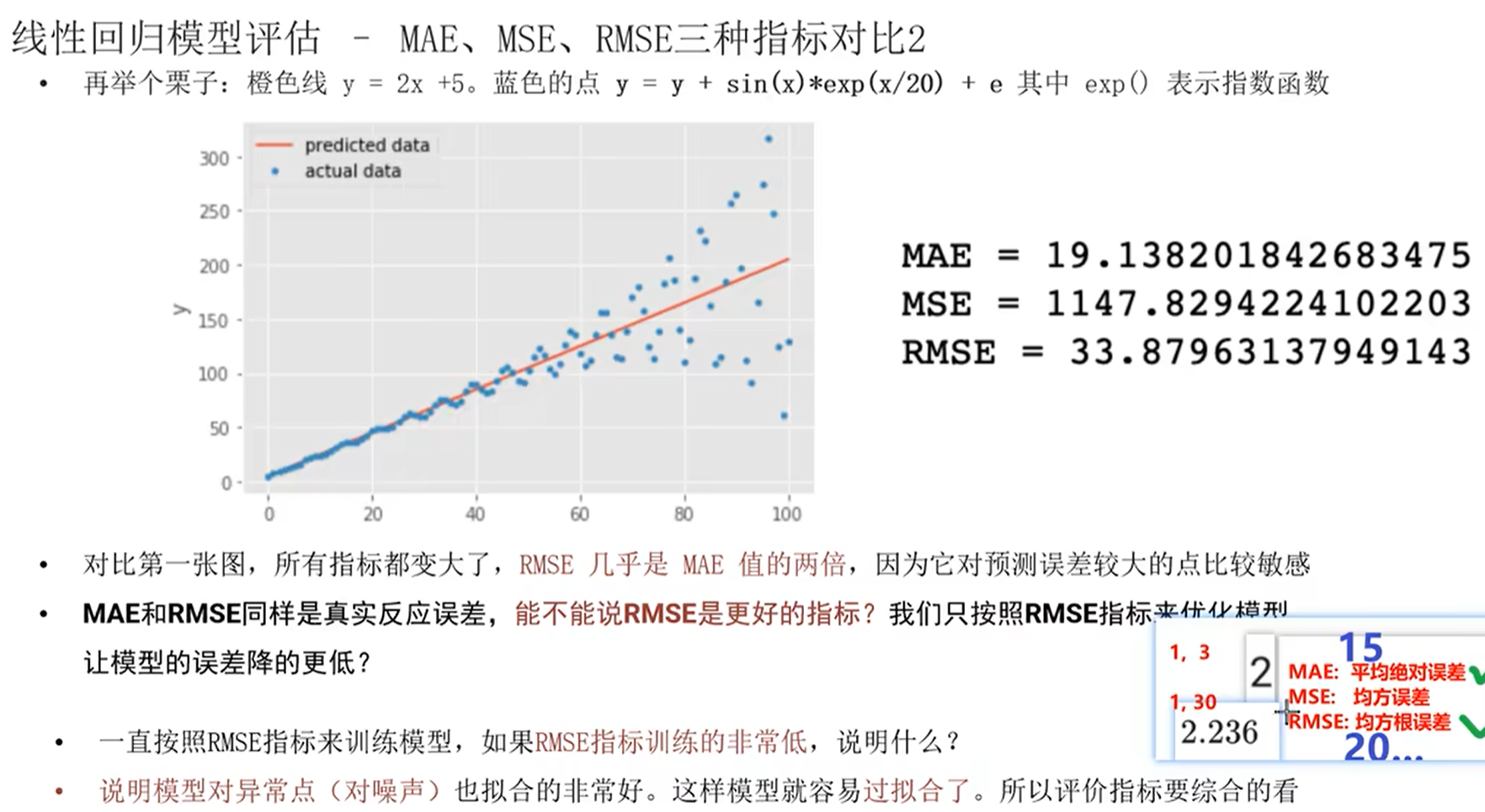
总结
- 一般使用 MAE 和 RMSE 这两个指标
MAE 反映的是“真实”的平均误差,RMSE 会将误差大的数据点放大
MAE 不能体现出误差大的数据点,RMSE 放大了大误差数据点对指标的影响,但对异常数据比较敏感
- 综合结论
都能反映出预测值和真实值之间的误差
MAE 对误差大小不敏感
RMSE 会放大预测误差较大的样本的影响
RMSE 对异常数据敏感
4.线性回归正规方程API和梯度下降API
sklearn.linear_model.LinearRegression
波士顿房价预测
1.属性信息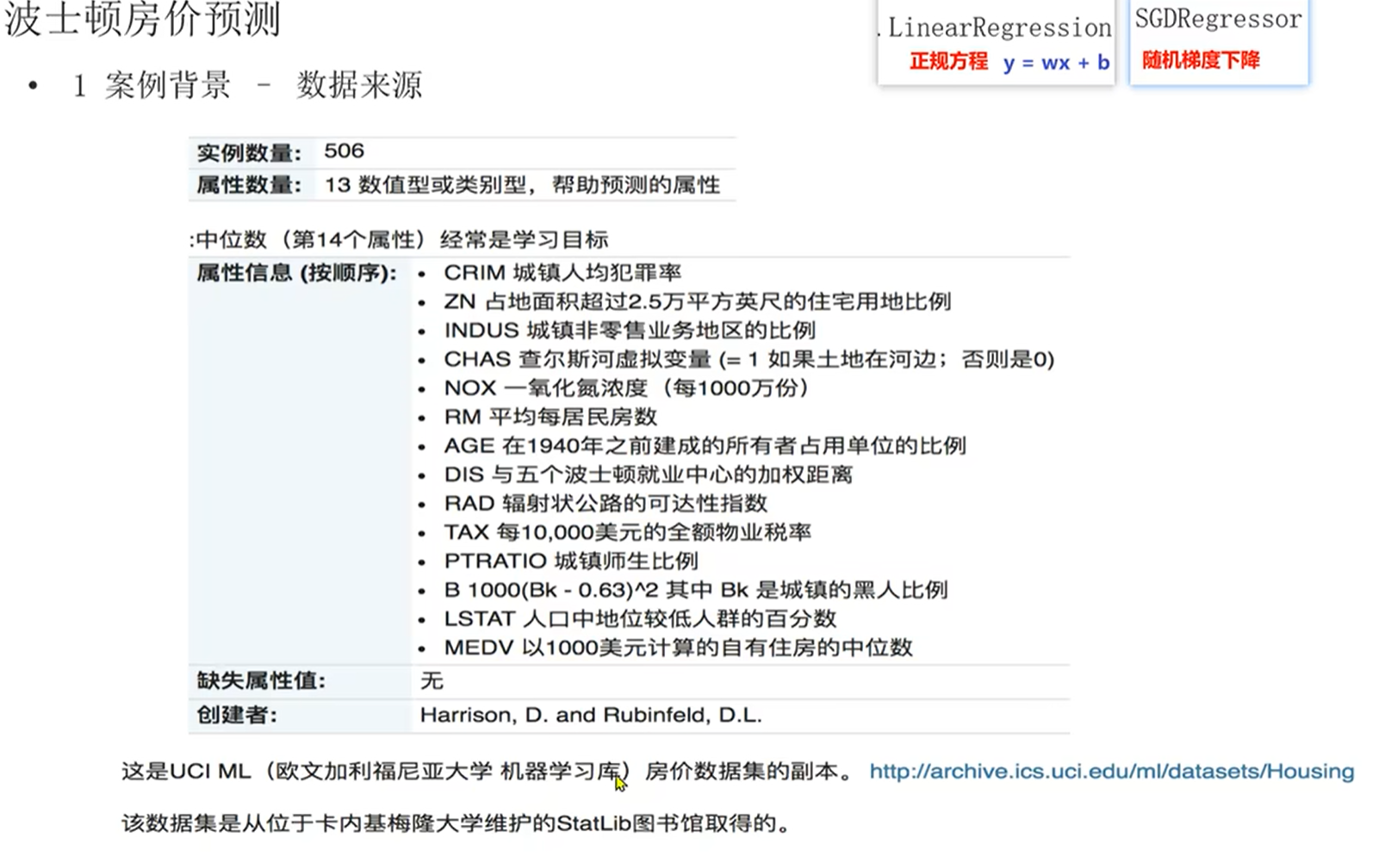
属性:13
实例数量:506
正规方程法求解API
"""
案例
    演示 正规方程法 线性回归对象 完成 波士顿房价预测

回顾
    线性回归∈ 有监督信息 有特征 有标签  目标是连续的
    线性回归分类
        一元线性回归:1个特征列,一个标签列
        多元线性回归:多个特征列,一个标签列
    大白话解释
        他是用线性公式来描述特征和标签之间的关系的,方便做预测,公示如下
        一元线性回归:y=w×x+b
        多元线性回归:y=w1x1+w2x2+...+b   = wᵀx+b
    如何评估线性回归模型的好坏
        思路
            预测值和正式值之间的误差,误差越小,模型越好
        具体的方案
            1.最小二乘   每个样本误差平方和
            2.均方误差   平均每个样本误差平方和
            3.均方根误差  平均每个样本误差的平方根
            4.平均绝对误差  每个样本误差绝对值和
    如何让损失函数最小
        思路1:梯度下降法 → 全梯度下降FGD 随机梯度下降SGD 小批量梯度下降Min-Batch 随机平均梯度下降SAG
        思路2:正规方程法

    机器学习开发流程
        1.加载数据
        2.数据预处理
        3.特征工程
        4.模型训练
        5.模型预测
        6.模型评估

"""
# from sklearn.datasets import load_boston        #数据
from sklearn.preprocessing import StandardScaler    #特征处理
from sklearn.model_selection import train_test_split    #数据集切分
from sklearn.linear_model import LinearRegression   #模型
from sklearn.metrics import mean_squared_error, mean_absolute_error, root_mean_squared_error  # 评估

import pandas as pd
import numpy as np

# 1. 加载数据
boston = pd.read_csv(r'D:\workspace\worksqace_python\ML\day01\data\boston.csv')
print(boston.head())
data = boston.iloc[:, :-1].values
target = boston.iloc[:, -1].values
print(f'特征:{data.shape}')
print(f'标签:{target.shape}')
print(f'特征数据:{data[:5]}')
print(f'标签数据:{target[:5]}')

# 2. 数据预处理
x_train, x_test, y_train, y_test = train_test_split(data, target, test_size=0.2, random_state=22)

# 3. 特征工程
# 3.1 数据标准化
transfer = StandardScaler()
x_train = transfer.fit_transform(x_train)
x_test = transfer.transform(x_test)

# 4.模型训练
# 4.1 创建 线性回归 正规方程 模型对象
# 参数:fit_intercept= True  是否计算截距
estimator = LinearRegression(fit_intercept= True)
# 4.2 模型训练
estimator.fit(x_train, y_train)
# 4.3 打印模型计算出的w(权重,weight)和b bais偏置
print(f'w:{estimator.coef_}')
print(f'b:{estimator.intercept_}')

# 5.模型预测
y_pre = estimator.predict(x_test)
print(f'预测结果:{y_pre}')

# 6. 模型评估
print(f'均方误差:{mean_squared_error(y_test, y_pre)}')
print(f'均方根误差:{root_mean_squared_error(y_test, y_pre)}')
print(f'平均绝对误差:{mean_absolute_error(y_test, y_pre)}')
随机梯度下降API
"""
案例
    演示 随机梯度下降法 线性回归对象 完成 波士顿房价预测

回顾
    线性回归∈ 有监督信息 有特征 有标签  目标是连续的
    线性回归分类
        一元线性回归:1个特征列,一个标签列
        多元线性回归:多个特征列,一个标签列
    大白话解释
        他是用线性公式来描述特征和标签之间的关系的,方便做预测,公示如下
        一元线性回归:y=w×x+b
        多元线性回归:y=w1x1+w2x2+...+b   = wᵀx+b
    如何评估线性回归模型的好坏
        思路
            预测值和正式值之间的误差,误差越小,模型越好
        具体的方案
            1.最小二乘   每个样本误差平方和
            2.均方误差   平均每个样本误差平方和
            3.均方根误差  平均每个样本误差的平方根
            4.平均绝对误差  每个样本误差绝对值和
    如何让损失函数最小
        思路1:梯度下降法 → 全梯度下降FGD 随机梯度下降SGD 小批量梯度下降Min-Batch 随机平均梯度下降SAG
        思路2:正规方程法

    机器学习开发流程
        1.加载数据
        2.数据预处理
        3.特征工程
        4.模型训练
        5.模型预测
        6.模型评估

"""
from sklearn.preprocessing import StandardScaler    #特征处理
from sklearn.model_selection import train_test_split    #数据集切分
from sklearn.linear_model import SGDRegressor   #模型
from sklearn.metrics import mean_squared_error, mean_absolute_error, root_mean_squared_error  # 评估

import pandas as pd
import numpy as np

# 1. 加载数据
boston = pd.read_csv(r'D:\workspace\worksqace_python\ML\day01\data\boston.csv')
print(boston.head())
data = boston.iloc[:, :-1].values
target = boston.iloc[:, -1].values
print(f'特征:{data.shape}')
print(f'标签:{target.shape}')
print(f'特征数据:{data[:5]}')
print(f'标签数据:{target[:5]}')


# 2.数据预处理
x_train, x_test, y_train, y_test = train_test_split(data, target, test_size=0.2, random_state=22)

# 3.特征工程
# 3.1 特征处理
transfer = StandardScaler()
x_train = transfer.fit_transform(x_train)
x_test = transfer.transform(x_test)


# 4.模型训练
# 4.1 创建梯度下降  线性回归模型对象
# 参1:是否需要截距
# 参2:学习率模式  常量 不会发生改变
# 参3:学习率
estimator = SGDRegressor(fit_intercept=True, learning_rate='constant', eta0=0.01)
estimator.fit(x_train, y_train)


# 5.模型预测
y_pre = estimator.predict(x_test)


# 6.模型评估
# MSE 均方误差  每个误差的平方和/样本数
print(f'均方误差:{mean_squared_error(y_test, y_pre)}') #参1:测试集的真实标签 参2:预测值
# RMSE 均方根误差   平均每个误差的平方根
print(f'均方根误差:{root_mean_squared_error(y_test, y_pre)}')
# MAE 平均绝对误差 每个误差绝对值和/样本数
print(f'平均绝对误差:{mean_absolute_error(y_test, y_pre)}')
5.欠拟合和过拟合
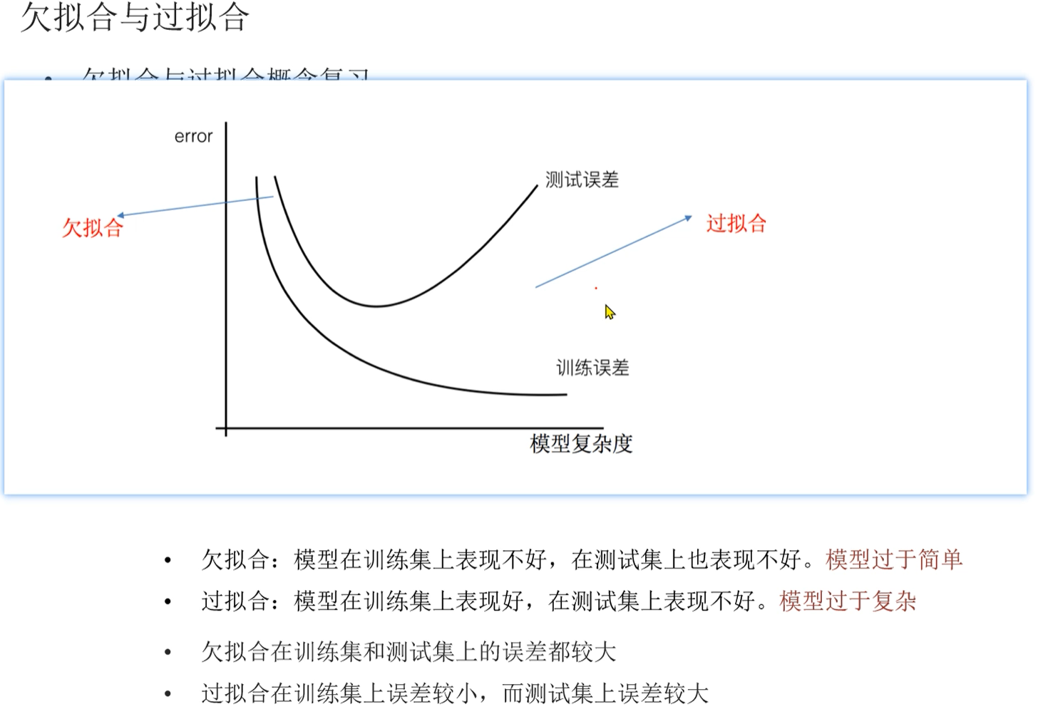
"""
案例
    演示 欠拟合,正好拟合,过拟合  L1正则 L2正则

回顾
    欠拟合    模型在训练集 和 测试集  表现效果都不好
    正好拟合   模型在训练集 和 测试集表现效果都很好
    过拟合     模型在 训练集 表现很好  测试集表现不好

"""
import numpy as np
from matplotlib import pyplot as plt
from sklearn.metrics import mean_squared_error, mean_absolute_error, root_mean_squared_error
from sklearn.linear_model import Ridge, RidgeCV, LinearRegression
import random

# 1.定义函数 模拟:欠拟合
def dm01_under_fitting():
    # 1.准备数据
    # 1.1 指定随机种子,则每次生成噪声的数据都是固定的
    np.random.seed(22)
    # 1.2 随机生成x轴  100个数据,模拟:特征
    x = np.random.uniform(-3,3,100) #参1:最小值,参2:最大值,参3:数据个数
    # 1.3 基于x轴值,通过线性公式,生成y轴  100个数据,模拟标签
    # 线性公式:y=kx+b = 0.5x²+2+噪声
    y = 0.5*x**2 + 2 + np.random.normal(0,1,100) #参1:均值,参2:标准差,参3:数据个数
    # 1.4 查看生成的x轴和y轴的数据
    print(f'特征x:{x}')
    print(f'标签y:{y}')


    # 2. 数据预处理,把x轴转成 多行1列的形式
    X=x.reshape(-1,1)
    # print(f'特征X:{X}')

    # 3. 特征工程,这里不做了,直接用100条数据,先训练,后预测
    # 4. 模型训练
    # 4.1 创建模型对象
    estimator = LinearRegression()

    # 4.2 模型训练
    estimator.fit(X,y)

    # 5.模型预测
    y_pre = estimator.predict(X)

    # 6.模型评估
    print(f'均方误差:{mean_squared_error(y,y_pre)}')
    print(f'均方根误差:{root_mean_squared_error(y,y_pre)}')
    print(f'平均绝对误差:{mean_absolute_error(y,y_pre)}')

    # 7.可视化
    plt.scatter(x,y)        #以散点图的形式绘制真实值
    plt.plot(x,y_pre,color='red')   #以线图绘制预测值

    plt.show()

# 2.定义函数 模拟:正好拟合
def dm02_just_fitting():
    # 1.准备数据
    # 1.1 指定随机种子,则每次生成噪声的数据都是固定的
    np.random.seed(23)
    # 1.2 随机生成x轴  100个数据,模拟:特征
    x = np.random.uniform(-3, 3, 100)  # 参1:最小值,参2:最大值,参3:数据个数
    # 1.3 基于x轴值,通过线性公式,生成y轴  100个数据,模拟标签
    # 线性公式:y=kx+b = 0.5x²+2+噪声
    y = 0.5 * x ** 2 +x+ 2 + np.random.normal(0, 1, 100)  # 参1:均值,参2:标准差,参3:数据个数
    # 1.4 查看生成的x轴和y轴的数据
    print(f'特征x:{x}')
    print(f'标签y:{y}')

    # 2. 数据预处理,把x轴转成 多行1列的形式
    # 2.1 把上述的x轴  转成多行1列的数据
    X = x.reshape(-1, 1)
    # print(f'特征X:{X}')

    # 2.2 因为目前特征只有一列,模型过于简单,会出现欠拟合的问题,我们增加1列特征值,从而增加模型复杂度
    # 即:把数据从[[1],[2],[3],[4],[5]]→[[1,1],[2,4],[3,9],[4,16],[5,25]]
    X2 = np.hstack([X,X**2]) #把x轴数据转成多列数据 模拟特征


    # 3. 特征工程,这里不做了,直接用100条数据,先训练,后预测
    # 4. 模型训练
    # 4.1 创建模型对象
    estimator = LinearRegression()

    # 4.2 模型训练
    estimator.fit(X2, y)

    # 5.模型预测
    y_pre = estimator.predict(X2)

    # 6.模型评估
    print(f'均方误差:{mean_squared_error(y, y_pre)}')
    print(f'均方根误差:{root_mean_squared_error(y, y_pre)}')
    print(f'平均绝对误差:{mean_absolute_error(y, y_pre)}')

    # 7.可视化
    plt.scatter(x, y)  # 以散点图的形式绘制真实值
    plt.plot(np.sort(x), y_pre[np.argsort(x)], color='red')  # 以线图绘制预测值

    plt.show()

# 3. 定义函数 模拟过拟合
def dm03_over_fitting():
    # 1.准备数据
    # 1.1 指定随机种子,则每次生成噪声的数据都是固定的
    np.random.seed(23)
    # 1.2 随机生成x轴  100个数据,模拟:特征
    x = np.random.uniform(-3, 3, 100)  # 参1:最小值,参2:最大值,参3:数据个数
    # 1.3 基于x轴值,通过线性公式,生成y轴  100个数据,模拟标签
    # 线性公式:y=kx+b = 0.5x²+2+噪声
    y = 0.5 * x ** 2 + x + 2 + np.random.normal(0, 1, 100)  # 参1:均值,参2:标准差,参3:数据个数
    # 1.4 查看生成的x轴和y轴的数据
    print(f'特征x:{x}')
    print(f'标签y:{y}')

    # 2. 数据预处理,把x轴转成 多行1列的形式
    # 2.1 把上述的x轴  转成多行1列的数据
    X = x.reshape(-1, 1)
    # print(f'特征X:{X}')

    # 2.2 因为目前特征只有一列,模型过于简单,会出现欠拟合的问题,我们增加9列特征值,从而增加模型复杂度
    # 即:把数据从[[1],[2],[3],[4],[5]]→[[1,1**2,1**3,1**4,1**5...],[2,2**2,2**3,2**4,2**5],[3,9],[4,16],[5,25]]
    X2 = np.hstack([X, X ** 2, X ** 3, X ** 4, X ** 5, X ** 6, X ** 7, X ** 8, X ** 9])  # 把x轴数据转成多列数据 模拟特征

    # 3. 特征工程,这里不做了,直接用100条数据,先训练,后预测
    # 4. 模型训练
    # 4.1 创建模型对象
    estimator = LinearRegression()

    # 4.2 模型训练
    estimator.fit(X2, y)

    # 5.模型预测
    y_pre = estimator.predict(X2)

    # 6.模型评估
    print(f'均方误差:{mean_squared_error(y, y_pre)}')
    print(f'均方根误差:{root_mean_squared_error(y, y_pre)}')
    print(f'平均绝对误差:{mean_absolute_error(y, y_pre)}')

    # 7.可视化
    plt.scatter(x, y)  # 以散点图的形式绘制真实值
    plt.plot(np.sort(x), y_pre[np.argsort(x)], color='red')  # 以线图绘制预测值

    plt.show()
if __name__ == '__main__':
    dm01_under_fitting()
    dm02_just_fitting()
    dm03_over_fitting()
6.欠拟合与过拟合 --出现原因和解决方案
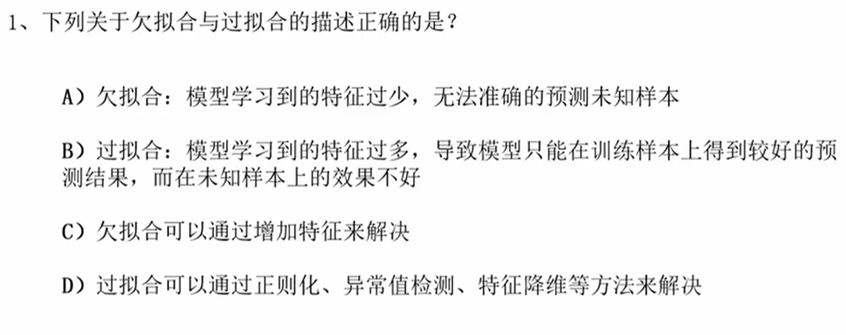
1.过拟合出现原因
- 原始特征过多,存在一些嘈杂特征,模型过于复杂是因为模型尝试去兼顾各个测试数据点
2.过拟合解决办法
- 重新清洗数据
- 增大数据的训练量
- 正则化
- 减少特征维度,防止维灾难
3.正则化概念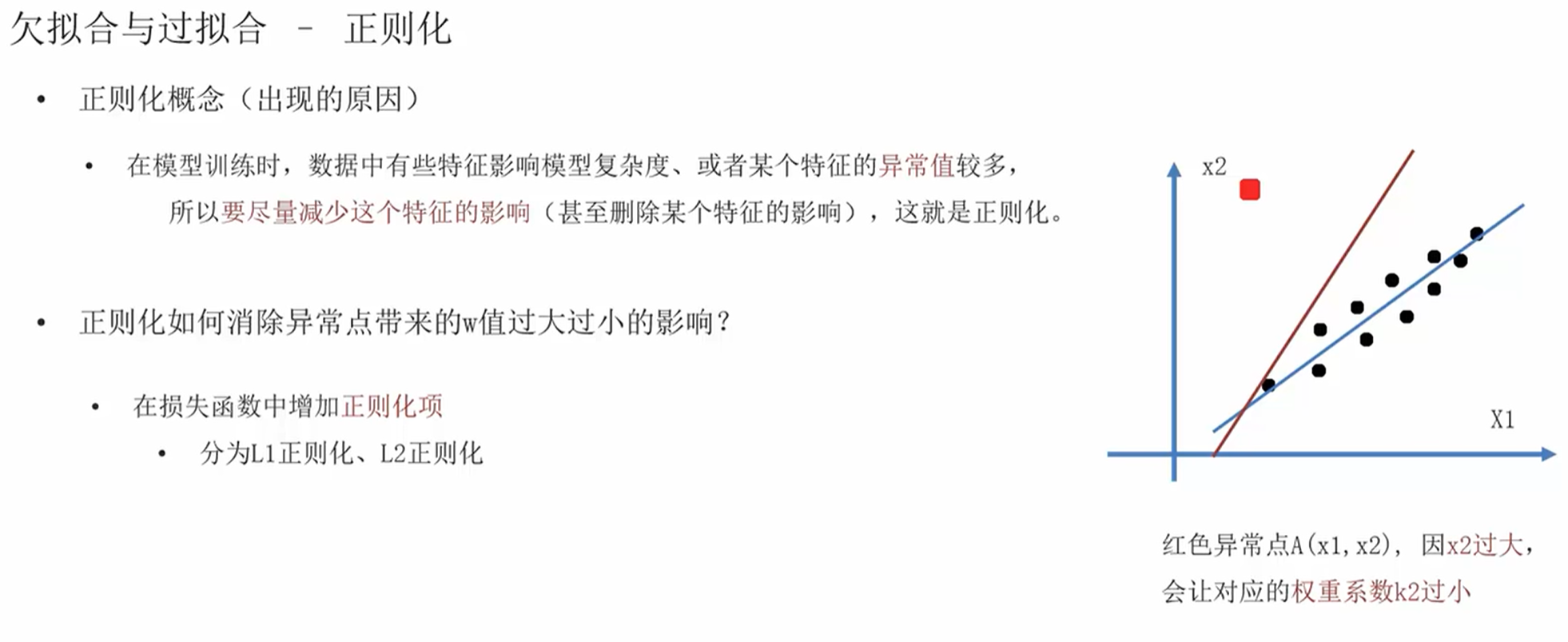
4.L1正则化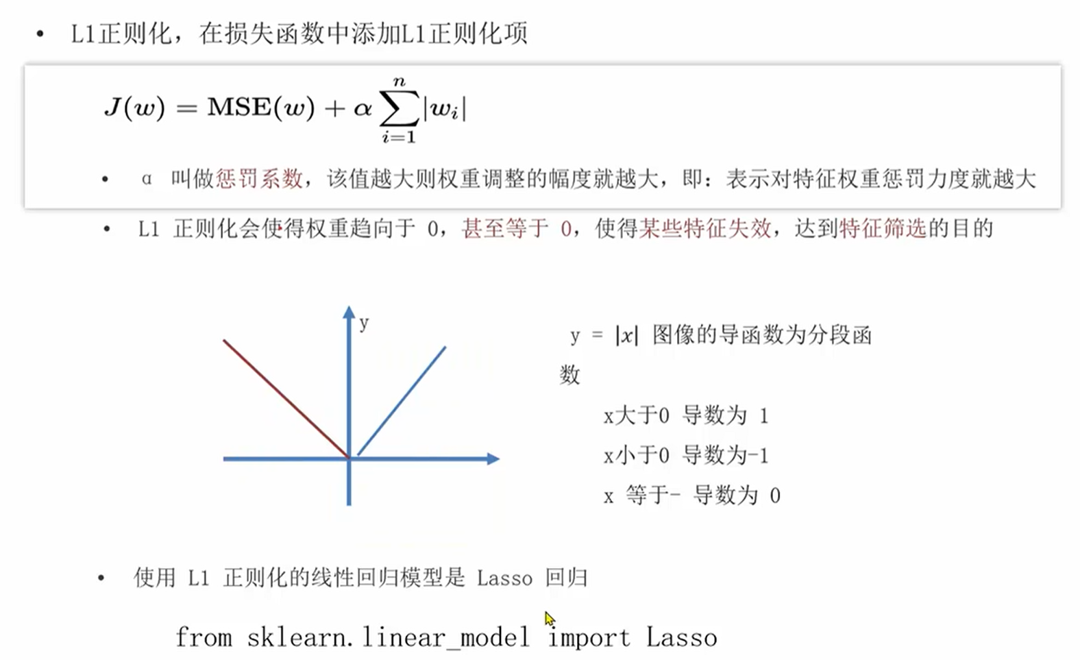
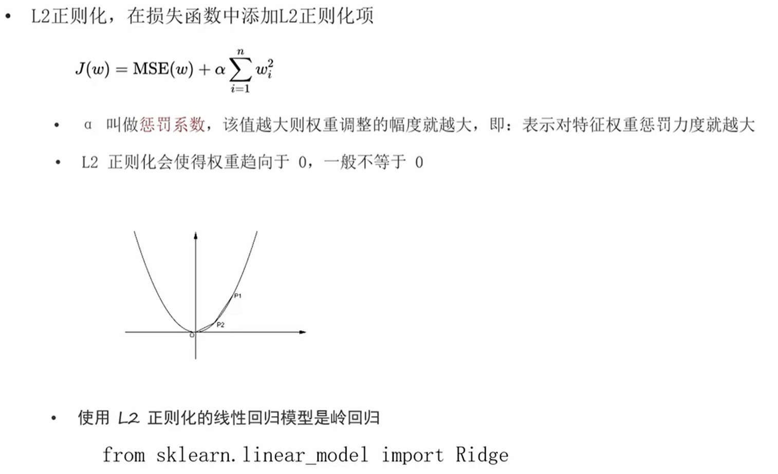
"""
案例
    演示 欠拟合,正好拟合,过拟合  L1正则 L2正则

回顾
    欠拟合    模型在训练集 和 测试集  表现效果都不好
    正好拟合   模型在训练集 和 测试集表现效果都很好
    过拟合     模型在 训练集 表现很好  测试集表现不好

过拟合,欠拟合解释
    产生原因
        欠拟合:模型简单
        过拟合:模型复杂
    解决方案
        欠拟合:增加特征,从而增加模型复杂度
        过拟合:减少模型复杂度,手动减少特征,L1和L2正则化
L1和L2化介绍
    目的/思路
        都是基于 惩罚系数 来修改特征列的权重的,惩罚系数越大,则修改力度就越大,对应的权重就越小
    区别
        L1正则化,可以实现让权重为0,从而达到特征选择的目的
        L2正则化,只能让权重无限趋近于0,但不能为0
    大白话:
        我要去爬山,带了个包,装了:登山杖,水,面包,衣服,鞋子  包装不下
        L1正则化:不带雨伞鞋子
        L2正则化:换一个大包,还是那些物品,空间占用权重变小了
"""
import numpy as np
from matplotlib import pyplot as plt
from sklearn.metrics import mean_squared_error, mean_absolute_error, root_mean_squared_error
from sklearn.linear_model import Ridge, RidgeCV, LinearRegression, Lasso
import random

# 1.定义函数 模拟:欠拟合
def dm01_under_fitting():
    # 1.准备数据
    # 1.1 指定随机种子,则每次生成噪声的数据都是固定的
    np.random.seed(22)
    # 1.2 随机生成x轴  100个数据,模拟:特征
    x = np.random.uniform(-3,3,100) #参1:最小值,参2:最大值,参3:数据个数
    # 1.3 基于x轴值,通过线性公式,生成y轴  100个数据,模拟标签
    # 线性公式:y=kx+b = 0.5x²+2+噪声
    y = 0.5*x**2 + 2 + np.random.normal(0,1,100) #参1:均值,参2:标准差,参3:数据个数
    # 1.4 查看生成的x轴和y轴的数据
    print(f'特征x:{x}')
    print(f'标签y:{y}')


    # 2. 数据预处理,把x轴转成 多行1列的形式
    X=x.reshape(-1,1)
    # print(f'特征X:{X}')

    # 3. 特征工程,这里不做了,直接用100条数据,先训练,后预测
    # 4. 模型训练
    # 4.1 创建模型对象
    estimator = LinearRegression()

    # 4.2 模型训练
    estimator.fit(X,y)

    # 5.模型预测
    y_pre = estimator.predict(X)

    # 6.模型评估
    print(f'均方误差:{mean_squared_error(y,y_pre)}')
    print(f'均方根误差:{root_mean_squared_error(y,y_pre)}')
    print(f'平均绝对误差:{mean_absolute_error(y,y_pre)}')

    # 7.可视化
    plt.scatter(x,y)        #以散点图的形式绘制真实值
    plt.plot(x,y_pre,color='red')   #以线图绘制预测值

    plt.show()

# 2.定义函数 模拟:正好拟合
def dm02_just_fitting():
    # 1.准备数据
    # 1.1 指定随机种子,则每次生成噪声的数据都是固定的
    np.random.seed(23)
    # 1.2 随机生成x轴  100个数据,模拟:特征
    x = np.random.uniform(-3, 3, 100)  # 参1:最小值,参2:最大值,参3:数据个数
    # 1.3 基于x轴值,通过线性公式,生成y轴  100个数据,模拟标签
    # 线性公式:y=kx+b = 0.5x²+2+噪声
    y = 0.5 * x ** 2 +x+ 2 + np.random.normal(0, 1, 100)  # 参1:均值,参2:标准差,参3:数据个数
    # 1.4 查看生成的x轴和y轴的数据
    print(f'特征x:{x}')
    print(f'标签y:{y}')

    # 2. 数据预处理,把x轴转成 多行1列的形式
    # 2.1 把上述的x轴  转成多行1列的数据
    X = x.reshape(-1, 1)
    # print(f'特征X:{X}')

    # 2.2 因为目前特征只有一列,模型过于简单,会出现欠拟合的问题,我们增加1列特征值,从而增加模型复杂度
    # 即:把数据从[[1],[2],[3],[4],[5]]→[[1,1],[2,4],[3,9],[4,16],[5,25]]
    X2 = np.hstack([X,X**2]) #把x轴数据转成多列数据 模拟特征


    # 3. 特征工程,这里不做了,直接用100条数据,先训练,后预测
    # 4. 模型训练
    # 4.1 创建模型对象
    estimator = LinearRegression()

    # 4.2 模型训练
    estimator.fit(X2, y)

    # 5.模型预测
    y_pre = estimator.predict(X2)

    # 6.模型评估
    print(f'均方误差:{mean_squared_error(y, y_pre)}')
    print(f'均方根误差:{root_mean_squared_error(y, y_pre)}')
    print(f'平均绝对误差:{mean_absolute_error(y, y_pre)}')

    # 7.可视化
    plt.scatter(x, y)  # 以散点图的形式绘制真实值
    plt.plot(np.sort(x), y_pre[np.argsort(x)], color='red')  # 以线图绘制预测值

    plt.show()

# 3. 定义函数 模拟过拟合
def dm03_over_fitting():
    # 1.准备数据
    # 1.1 指定随机种子,则每次生成噪声的数据都是固定的
    np.random.seed(23)
    # 1.2 随机生成x轴  100个数据,模拟:特征
    x = np.random.uniform(-3, 3, 100)  # 参1:最小值,参2:最大值,参3:数据个数
    # 1.3 基于x轴值,通过线性公式,生成y轴  100个数据,模拟标签
    # 线性公式:y=kx+b = 0.5x²+2+噪声
    y = 0.5 * x ** 2 + x + 2 + np.random.normal(0, 1, 100)  # 参1:均值,参2:标准差,参3:数据个数
    # 1.4 查看生成的x轴和y轴的数据
    print(f'特征x:{x}')
    print(f'标签y:{y}')

    # 2. 数据预处理,把x轴转成 多行1列的形式
    # 2.1 把上述的x轴  转成多行1列的数据
    X = x.reshape(-1, 1)
    # print(f'特征X:{X}')

    # 2.2 因为目前特征只有一列,模型过于简单,会出现欠拟合的问题,我们增加9列特征值,从而增加模型复杂度
    # 即:把数据从[[1],[2],[3],[4],[5]]→[[1,1**2,1**3,1**4,1**5...],[2,2**2,2**3,2**4,2**5],[3,9],[4,16],[5,25]]
    X2 = np.hstack([X, X ** 2, X ** 3, X ** 4, X ** 5, X ** 6, X ** 7, X ** 8, X ** 9])  # 把x轴数据转成多列数据 模拟特征

    # 3. 特征工程,这里不做了,直接用100条数据,先训练,后预测
    # 4. 模型训练
    # 4.1 创建模型对象
    estimator = LinearRegression()

    # 4.2 模型训练
    estimator.fit(X2, y)

    # 5.模型预测
    y_pre = estimator.predict(X2)

    # 6.模型评估
    print(f'均方误差:{mean_squared_error(y, y_pre)}')
    print(f'均方根误差:{root_mean_squared_error(y, y_pre)}')
    print(f'平均绝对误差:{mean_absolute_error(y, y_pre)}')

    # 7.可视化
    plt.scatter(x, y)  # 以散点图的形式绘制真实值
    plt.plot(np.sort(x), y_pre[np.argsort(x)], color='red')  # 以线图绘制预测值

    plt.show()

# 4.定义函数,模拟L1正则化
def dm04_l1_regularization():
    # 1.准备数据
    # 1.1 指定随机种子,则每次生成噪声的数据都是固定的
    np.random.seed(23)
    # 1.2 随机生成x轴  100个数据,模拟:特征
    x = np.random.uniform(-3, 3, 100)  # 参1:最小值,参2:最大值,参3:数据个数
    # 1.3 基于x轴值,通过线性公式,生成y轴  100个数据,模拟标签
    # 线性公式:y=kx+b = 0.5x²+2+噪声
    y = 0.5 * x ** 2 + x + 2 + np.random.normal(0, 1, 100)  # 参1:均值,参2:标准差,参3:数据个数
    # 1.4 查看生成的x轴和y轴的数据
    print(f'特征x:{x}')
    print(f'标签y:{y}')

    # 2. 数据预处理,把x轴转成 多行1列的形式
    # 2.1 把上述的x轴  转成多行1列的数据
    X = x.reshape(-1, 1)
    # print(f'特征X:{X}')

    # 2.2 因为目前特征只有一列,模型过于简单,会出现欠拟合的问题,我们增加9列特征值,从而增加模型复杂度
    # 即:把数据从[[1],[2],[3],[4],[5]]→[[1,1**2,1**3,1**4,1**5...],[2,2**2,2**3,2**4,2**5],[3,9],[4,16],[5,25]]
    X2 = np.hstack([X, X ** 2, X ** 3, X ** 4, X ** 5, X ** 6, X ** 7, X ** 8, X ** 9])  # 把x轴数据转成多列数据 模拟特征

    # 3. 特征工程,这里不做了,直接用100条数据,先训练,后预测
    # 4. 模型训练
    # 4.1 创建正则化
    estimator = Lasso(alpha=0.1) #alpha:正则化参数   惩罚系数 默认是1

    # 4.2 模型训练
    estimator.fit(X2, y)

    # 5.模型预测
    y_pre = estimator.predict(X2)

    # 6.模型评估
    print(f'均方误差:{mean_squared_error(y, y_pre)}')
    print(f'均方根误差:{root_mean_squared_error(y, y_pre)}')
    print(f'平均绝对误差:{mean_absolute_error(y, y_pre)}')

    # 7.可视化
    plt.scatter(x, y)  # 以散点图的形式绘制真实值
    plt.plot(np.sort(x), y_pre[np.argsort(x)], color='red')  # 以线图绘制预测值

    plt.show()
# 5.定义函数,模拟L2正则化
def dm05_l1_regularization():
    # 1.准备数据
    # 1.1 指定随机种子,则每次生成噪声的数据都是固定的
    np.random.seed(23)
    # 1.2 随机生成x轴  100个数据,模拟:特征
    x = np.random.uniform(-3, 3, 100)  # 参1:最小值,参2:最大值,参3:数据个数
    # 1.3 基于x轴值,通过线性公式,生成y轴  100个数据,模拟标签
    # 线性公式:y=kx+b = 0.5x²+2+噪声
    y = 0.5 * x ** 2 + x + 2 + np.random.normal(0, 1, 100)  # 参1:均值,参2:标准差,参3:数据个数
    # 1.4 查看生成的x轴和y轴的数据
    print(f'特征x:{x}')
    print(f'标签y:{y}')

    # 2. 数据预处理,把x轴转成 多行1列的形式
    # 2.1 把上述的x轴  转成多行1列的数据
    X = x.reshape(-1, 1)
    # print(f'特征X:{X}')

    # 2.2 因为目前特征只有一列,模型过于简单,会出现欠拟合的问题,我们增加9列特征值,从而增加模型复杂度
    # 即:把数据从[[1],[2],[3],[4],[5]]→[[1,1**2,1**3,1**4,1**5...],[2,2**2,2**3,2**4,2**5],[3,9],[4,16],[5,25]]
    X2 = np.hstack([X, X ** 2, X ** 3, X ** 4, X ** 5, X ** 6, X ** 7, X ** 8, X ** 9])  # 把x轴数据转成多列数据 模拟特征

    # 3. 特征工程,这里不做了,直接用100条数据,先训练,后预测
    # 4. 模型训练
    # 4.1 创建正则化
    estimator = Ridge(alpha=10) #alpha:正则化参数   惩罚系数 默认是1

    # 4.2 模型训练
    estimator.fit(X2, y)

    # 5.模型预测
    y_pre = estimator.predict(X2)

    # 6.模型评估
    print(f'均方误差:{mean_squared_error(y, y_pre)}')
    print(f'均方根误差:{root_mean_squared_error(y, y_pre)}')
    print(f'平均绝对误差:{mean_absolute_error(y, y_pre)}')

    # 7.可视化
    plt.scatter(x, y)  # 以散点图的形式绘制真实值
    plt.plot(np.sort(x), y_pre[np.argsort(x)], color='red')  # 以线图绘制预测值

    plt.show()

if __name__ == '__main__':
    # dm01_under_fitting()
    # dm02_just_fitting()
    # dm03_over_fitting()
    # dm04_l1_regularization()
    dm05_l1_regularization()
总结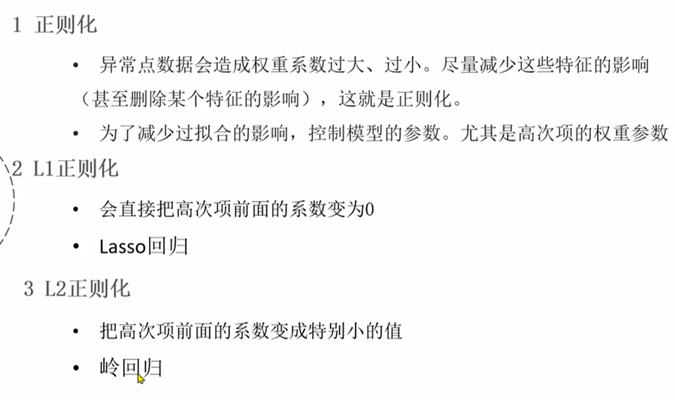
ABCD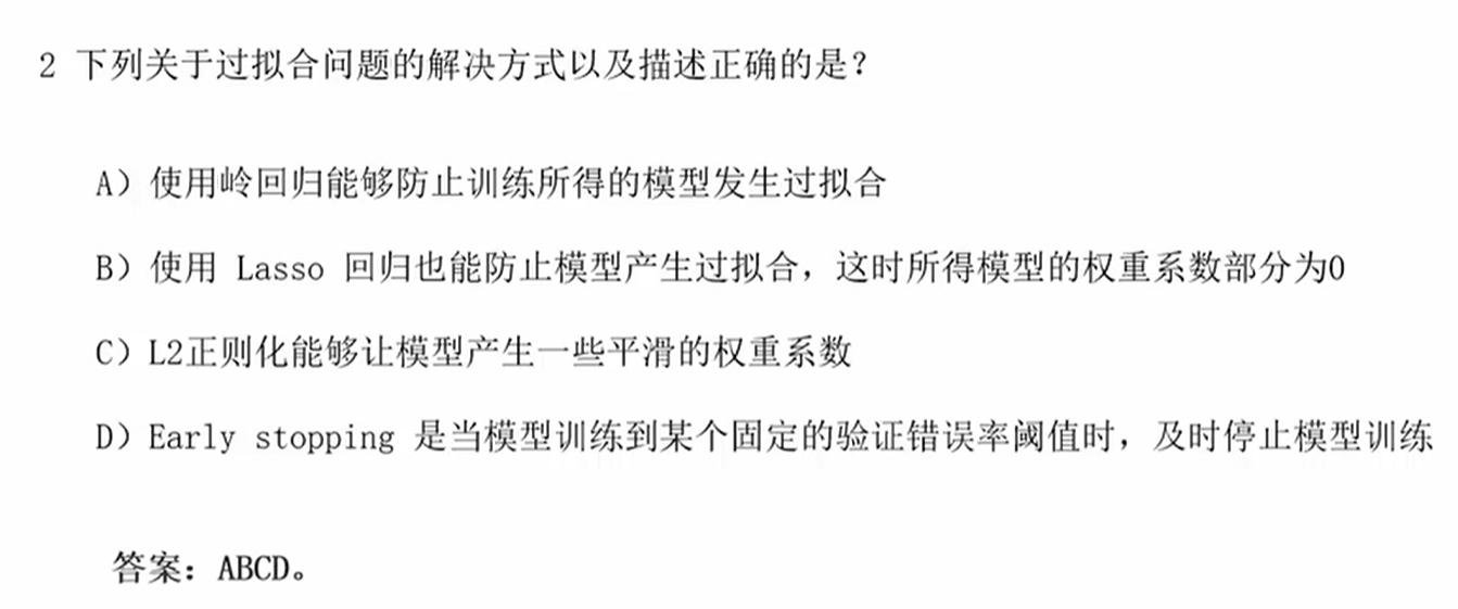
结束 重点是损失函数+梯度下降

Agent 垂直技术社区,欢迎活跃、内容共建。
更多推荐


 4
4 0
0- 0


 已为社区贡献9条内容

所有评论(0)