结构健康监测仿真-主题061-结构健康监测中的机器学习应用

kkchenkx

439人浏览 · 2026-05-02 07:19:30

kkchenkx · 2026-05-02 07:19:30 发布

结构健康监测仿真 - 主题061：结构健康监测中的机器学习应用

1. 引言

1.1 机器学习在SHM中的重要性

结构健康监测（Structural Health Monitoring, SHM）系统产生的数据量呈指数级增长，传统的基于物理模型的分析方法面临计算复杂度高、难以处理非线性问题等挑战。机器学习（Machine Learning, ML）作为一种数据驱动的方法，为SHM提供了新的解决方案。

机器学习在SHM中的核心价值体现在以下几个方面：

数据处理能力：现代SHM系统每天可产生GB甚至TB级的监测数据。机器学习算法能够自动从海量数据中提取有意义的特征，识别数据中的模式和规律，大大降低了人工分析的工作量。

非线性建模能力：结构的损伤行为往往表现出强烈的非线性特征，传统的线性模型难以准确描述。机器学习，特别是深度学习，具有强大的非线性映射能力，能够学习复杂的损伤演化规律。

自适应学习能力：机器学习模型可以根据新的监测数据不断更新和优化，适应结构服役过程中的性能退化，实现自适应的健康状态评估。

多源信息融合：SHM系统通常包含多种类型的传感器（加速度计、应变片、位移计等），机器学习能够有效地融合多源异构信息，提高损伤识别的准确性。

1.2 机器学习SHM的发展历程

机器学习在SHM中的应用经历了从简单到复杂、从浅层到深层的发展过程：

第一阶段（1990s-2000s）：传统机器学习方法

人工神经网络（ANN）用于损伤识别
支持向量机（SVM）用于分类问题
遗传算法用于优化传感器布置

第二阶段（2000s-2010s）：集成学习与核方法

随机森林、梯度提升树等集成方法
核主成分分析（KPCA）用于特征提取
隐马尔可夫模型（HMM）用于时序分析

第三阶段（2010s-至今）：深度学习时代

卷积神经网络（CNN）用于图像类损伤检测
循环神经网络（RNN/LSTM）用于时序数据分析
自编码器用于异常检测
生成对抗网络（GAN）用于数据增强

1.3 本主题学习目标

通过本主题的学习，读者将能够：

理解机器学习的基本原理和在SHM中的应用场景
掌握监督学习、无监督学习、深度学习在损伤识别中的具体方法
学会使用Python实现机器学习SHM算法
了解迁移学习等前沿技术在SHM中的应用
具备解决实际工程问题的能力

2. 机器学习基础理论

2.1 机器学习的基本概念

机器学习是人工智能的一个分支，其核心思想是让计算机通过数据学习规律，而不是通过明确的编程指令。在SHM中，机器学习的目标是从监测数据中学习结构的健康状态与损伤特征之间的关系。

基本定义：
给定训练数据集 $D = {(x_1, y_1), (x_2, y_2), ..., (x_n, y_n)}$ ，其中 $x_i$ 是输入特征（如传感器数据）， $y_i$ 是对应的标签（如健康/损伤状态）。机器学习的目标是找到一个函数 $f$ ，使得 $\approx y$ 。

学习类型：

监督学习（Supervised Learning）
- 训练数据包含输入和对应的标签
- 目标：学习从输入到输出的映射关系
- SHM应用：损伤分类、损伤程度评估、剩余寿命预测
无监督学习（Unsupervised Learning）
- 训练数据只有输入，没有标签
- 目标：发现数据中的内在结构
- SHM应用：异常检测、数据降维、聚类分析
半监督学习（Semi-supervised Learning）
- 训练数据包含少量标签数据和大量无标签数据
- 目标：利用无标签数据提高学习性能
- SHM应用：标签数据稀缺的损伤识别
强化学习（Reinforcement Learning）
- 通过与环境交互学习最优策略
- 目标：最大化累积奖励
- SHM应用：传感器优化布置、维护决策

2.2 特征工程与数据预处理

特征工程是机器学习中最重要的环节之一，直接影响模型的性能。在SHM中，原始传感器数据通常需要经过预处理才能用于机器学习。

数据预处理步骤：

数据清洗

import numpy as np
from scipy import signal

def clean_sensor_data(raw_data, threshold=3):
    """
    清洗传感器数据，去除异常值和噪声
    
    参数:
    raw_data: 原始传感器数据
    threshold: 异常值检测阈值（标准差的倍数）
    
    返回:
    cleaned_data: 清洗后的数据
    """
    # 去除趋势项
    detrended = signal.detrend(raw_data)
    
    # 使用Z-score方法检测异常值
    mean = np.mean(detrended)
    std = np.std(detrended)
    z_scores = np.abs((detrended - mean) / std)
    
    # 替换异常值
    cleaned_data = detrended.copy()
    cleaned_data[z_scores > threshold] = mean
    
    return cleaned_data

特征提取

时域特征：

均值： $\mu = \frac{1}{N}\sum_{i=1}^{N}x_i$
标准差： $\sigma = \sqrt{\frac{1}{N}\sum_{i=1}^{N}(x_i - \mu)^2}$
峰值： $P = \max(|x_i|)$
峰度： $\frac{1}{N}\sum_{i=1}^{N}\left(\frac{x_i - \mu}{\sigma}\right)^4$
偏度： $\frac{1}{N}\sum_{i=1}^{N}\left(\frac{x_i - \mu}{\sigma}\right)^3$

频域特征：

主频率：功率谱密度峰值对应的频率
频带能量：特定频带内的能量占比
频谱质心： $\frac{\sum_{k}f_k \cdot P_k}{\sum_{k}P_k}$

def extract_features(data, fs=1000):
    """
    提取时频域特征
    
    参数:
    data: 输入信号
    fs: 采样频率
    
    返回:
    features: 特征字典
    """
    features = {}
    
    # 时域特征
    features['mean'] = np.mean(data)
    features['std'] = np.std(data)
    features['max'] = np.max(np.abs(data))
    features['rms'] = np.sqrt(np.mean(data**2))
    features['kurtosis'] = np.mean((data - features['mean'])**4) / (features['std']**4)
    features['skewness'] = np.mean((data - features['mean'])**3) / (features['std']**3)
    
    # 频域特征
    fft = np.fft.fft(data)
    freqs = np.fft.fftfreq(len(data), 1/fs)
    psd = np.abs(fft)**2
    
    features['dominant_freq'] = freqs[np.argmax(psd[:len(psd)//2])]
    features['spectral_centroid'] = np.sum(freqs[:len(freqs)//2] * psd[:len(psd)//2]) / np.sum(psd[:len(psd)//2])
    
    return features

数据归一化

from sklearn.preprocessing import StandardScaler, MinMaxScaler

def normalize_features(features, method='standard'):
    """
    特征归一化
    
    参数:
    features: 特征矩阵
    method: 'standard'或'minmax'
    
    返回:
    normalized_features: 归一化后的特征
    scaler: 归一化器（用于后续数据转换）
    """
    if method == 'standard':
        scaler = StandardScaler()
    else:
        scaler = MinMaxScaler()
    
    normalized_features = scaler.fit_transform(features)
    return normalized_features, scaler

2.3 模型评估与验证

在SHM中，模型评估需要特别关注泛化能力，因为实际结构的损伤模式可能与训练数据不同。

评估指标：

分类问题
- 准确率（Accuracy）： $\frac{TP + TN}{TP + TN + FP + FN}$
- 精确率（Precision）： $\frac{TP}{TP + FP}$
- 召回率（Recall）： $\frac{TP}{TP + FN}$
- F1分数： $\cdot \frac{P \cdot R}{P + R}$
回归问题
- 均方误差（MSE）： $\frac{1}{n}\sum_{i=1}^{n}(y_i - \hat{y}_i)^2$
- 均方根误差（RMSE）： $\sqrt{MSE}$
- 决定系数（ $R^2$ ）： $R^2 = 1 - \frac{\sum(y_i - \hat{y}_i)^2}{\sum(y_i - \bar{y})^2}$

交叉验证：

from sklearn.model_selection import cross_val_score, StratifiedKFold

def evaluate_model(model, X, y, cv_folds=5):
    """
    使用交叉验证评估模型
    
    参数:
    model: 机器学习模型
    X: 特征矩阵
    y: 标签
    cv_folds: 交叉验证折数
    
    返回:
    scores: 各折的评估分数
    """
    cv = StratifiedKFold(n_splits=cv_folds, shuffle=True, random_state=42)
    scores = cross_val_score(model, X, y, cv=cv, scoring='accuracy')
    
    return {
        'mean': scores.mean(),
        'std': scores.std(),
        'scores': scores
    }

3. 监督学习在SHM中的应用

3.1 支持向量机（SVM）

支持向量机是一种强大的分类算法，在SHM中广泛用于损伤分类和定位。

基本原理：
SVM的目标是找到一个最优超平面，使得不同类别的数据点之间的间隔最大化。对于非线性可分问题，SVM使用核函数将数据映射到高维特征空间。

数学表述：
给定训练数据 $x_i, y_i)$ ，其中 $y_i \in \{-1, 1\}$ ，SVM求解以下优化问题：

$\min_{w, b} \frac{1}{2}||w||^2 + C\sum_{i=1}^{n}\max(0, 1 - y_i(w^T x_i + b))$

核函数选择：

线性核： $K(x, x') = x^T x'$
多项式核： $(\gamma x^T x' + r)^d$
RBF核： $\exp(-\gamma ||x - x'||^2)$

from sklearn.svm import SVC
from sklearn.model_selection import GridSearchCV

def train_svm_damage_classifier(X_train, y_train):
    """
    训练SVM损伤分类器
    
    参数:
    X_train: 训练特征
    y_train: 训练标签（0=健康，1=损伤）
    
    返回:
    model: 训练好的SVM模型
    """
    # 定义参数网格
    param_grid = {
        'C': [0.1, 1, 10, 100],
        'gamma': ['scale', 'auto', 0.001, 0.01, 0.1],
        'kernel': ['rbf', 'poly', 'linear']
    }
    
    # 使用网格搜索寻找最优参数
    svm = SVC(probability=True, random_state=42)
    grid_search = GridSearchCV(svm, param_grid, cv=5, scoring='accuracy', n_jobs=-1)
    grid_search.fit(X_train, y_train)
    
    print(f"最优参数: {grid_search.best_params_}")
    print(f"最佳交叉验证得分: {grid_search.best_score_:.4f}")
    
    return grid_search.best_estimator_

# 示例：使用SVM进行损伤分类
# model = train_svm_damage_classifier(X_train, y_train)
# y_pred = model.predict(X_test)

应用案例：
在一座斜拉桥的SHM系统中，使用SVM对加速度传感器数据进行分类，成功识别了拉索损伤、主梁损伤和支座损伤三种类型，分类准确率达到94.5%。

3.2 随机森林

随机森林是一种集成学习方法，通过构建多棵决策树并综合它们的预测结果来提高准确性。

算法优势：

能够处理高维数据
对噪声和异常值不敏感
能够评估特征重要性
不容易过拟合

from sklearn.ensemble import RandomForestClassifier
import matplotlib.pyplot as plt

def train_random_forest(X_train, y_train, n_estimators=100):
    """
    训练随机森林分类器
    
    参数:
    X_train: 训练特征
    y_train: 训练标签
    n_estimators: 树的数量
    
    返回:
    model: 训练好的模型
    feature_importance: 特征重要性
    """
    rf = RandomForestClassifier(
        n_estimators=n_estimators,
        max_depth=10,
        min_samples_split=5,
        random_state=42,
        n_jobs=-1
    )
    
    rf.fit(X_train, y_train)
    
    # 获取特征重要性
    feature_importance = rf.feature_importances_
    
    return rf, feature_importance

def plot_feature_importance(feature_names, importance, top_n=10):
    """
    可视化特征重要性
    
    参数:
    feature_names: 特征名称列表
    importance: 特征重要性数组
    top_n: 显示前N个重要特征
    """
    # 排序
    indices = np.argsort(importance)[::-1][:top_n]
    
    plt.figure(figsize=(10, 6))
    plt.bar(range(top_n), importance[indices], align='center')
    plt.xticks(range(top_n), [feature_names[i] for i in indices], rotation=45)
    plt.xlabel('特征')
    plt.ylabel('重要性')
    plt.title(f'前{top_n}个重要特征')
    plt.tight_layout()
    plt.savefig('feature_importance.png', dpi=150)
    plt.close()

3.3 梯度提升树（XGBoost/LightGBM）

梯度提升树是目前最流行的集成学习方法之一，在各类数据竞赛中表现出色。

XGBoost特点：

使用二阶泰勒展开近似损失函数
加入正则化项防止过拟合
支持并行计算
能够处理缺失值

import xgboost as xgb
from sklearn.metrics import classification_report

def train_xgboost_classifier(X_train, y_train, X_test, y_test):
    """
    训练XGBoost分类器
    
    参数:
    X_train, y_train: 训练数据
    X_test, y_test: 测试数据
    
    返回:
    model: 训练好的模型
    """
    # 创建DMatrix
    dtrain = xgb.DMatrix(X_train, label=y_train)
    dtest = xgb.DMatrix(X_test, label=y_test)
    
    # 设置参数
    params = {
        'objective': 'binary:logistic',
        'max_depth': 6,
        'learning_rate': 0.1,
        'subsample': 0.8,
        'colsample_bytree': 0.8,
        'eval_metric': 'auc',
        'seed': 42
    }
    
    # 训练模型
    model = xgb.train(
        params,
        dtrain,
        num_boost_round=100,
        evals=[(dtest, 'test')],
        early_stopping_rounds=10,
        verbose_eval=False
    )
    
    # 预测
    y_pred = (model.predict(dtest) > 0.5).astype(int)
    
    print("分类报告:")
    print(classification_report(y_test, y_pred))
    
    return model

4. 无监督学习与异常检测

4.1 主成分分析（PCA）

PCA是一种常用的降维技术，在SHM中用于特征提取和异常检测。

基本原理：
PCA通过线性变换将原始特征投影到新的坐标系，使得第一主成分方向上的方差最大，第二主成分与第一主成分正交且方差次大，以此类推。

数学推导：
给定数据矩阵 $\in \mathbb{R}^{n \times p}$ ，PCA求解协方差矩阵的特征值问题：

$\Sigma = \frac{1}{n-1}X^T X = V \Lambda V^T$

其中 $V$ 是特征向量矩阵， $\Lambda$ 是特征值对角矩阵。

from sklearn.decomposition import PCA
from sklearn.preprocessing import StandardScaler

def apply_pca_for_shm(data, n_components=0.95):
    """
    应用PCA进行降维和异常检测
    
    参数:
    data: 原始特征数据
    n_components: 保留的方差比例或组件数量
    
    返回:
    pca: PCA模型
    transformed_data: 降维后的数据
    reconstruction_error: 重构误差（用于异常检测）
    """
    # 标准化
    scaler = StandardScaler()
    data_scaled = scaler.fit_transform(data)
    
    # PCA
    pca = PCA(n_components=n_components)
    transformed_data = pca.fit_transform(data_scaled)
    
    # 重构
    reconstructed = pca.inverse_transform(transformed_data)
    reconstruction_error = np.mean((data_scaled - reconstructed)**2, axis=1)
    
    print(f"原始维度: {data.shape[1]}")
    print(f"降维后维度: {transformed_data.shape[1]}")
    print(f"解释方差比例: {np.sum(pca.explained_variance_ratio_):.4f}")
    
    return pca, transformed_data, reconstruction_error, scaler

def detect_anomalies_pca(reconstruction_error, threshold_percentile=95):
    """
    基于PCA重构误差进行异常检测
    
    参数:
    reconstruction_error: 重构误差
    threshold_percentile: 阈值百分位数
    
    返回:
    anomalies: 异常样本索引
    threshold: 异常阈值
    """
    threshold = np.percentile(reconstruction_error, threshold_percentile)
    anomalies = np.where(reconstruction_error > threshold)[0]
    
    print(f"异常阈值: {threshold:.4f}")
    print(f"检测到 {len(anomalies)} 个异常样本")
    
    return anomalies, threshold

4.2 自编码器（Autoencoder）

自编码器是一种神经网络，通过学习数据的压缩表示来进行无监督学习。

网络结构：

编码器：将输入映射到低维潜在空间
解码器：从潜在空间重构输入
损失函数：重构误差

import tensorflow as tf
from tensorflow.keras.models import Model
from tensorflow.keras.layers import Input, Dense

def build_autoencoder(input_dim, encoding_dim=10):
    """
    构建自编码器模型
    
    参数:
    input_dim: 输入维度
    encoding_dim: 编码维度
    
    返回:
    autoencoder: 完整自编码器
    encoder: 编码器部分
    """
    # 输入层
    input_layer = Input(shape=(input_dim,))
    
    # 编码器
    encoded = Dense(64, activation='relu')(input_layer)
    encoded = Dense(32, activation='relu')(encoded)
    encoded = Dense(encoding_dim, activation='relu')(encoded)
    
    # 解码器
    decoded = Dense(32, activation='relu')(encoded)
    decoded = Dense(64, activation='relu')(decoded)
    decoded = Dense(input_dim, activation='linear')(decoded)
    
    # 完整模型
    autoencoder = Model(input_layer, decoded)
    encoder = Model(input_layer, encoded)
    
    autoencoder.compile(optimizer='adam', loss='mse')
    
    return autoencoder, encoder

def train_autoencoder(autoencoder, X_train, X_val, epochs=100, batch_size=32):
    """
    训练自编码器
    
    参数:
    autoencoder: 自编码器模型
    X_train: 训练数据（健康状态数据）
    X_val: 验证数据
    epochs: 训练轮数
    batch_size: 批次大小
    
    返回:
    history: 训练历史
    """
    history = autoencoder.fit(
        X_train, X_train,
        epochs=epochs,
        batch_size=batch_size,
        validation_data=(X_val, X_val),
        verbose=0
    )
    
    return history

def detect_anomalies_autoencoder(autoencoder, data, threshold_percentile=95):
    """
    使用自编码器进行异常检测
    
    参数:
    autoencoder: 训练好的自编码器
    data: 测试数据
    threshold_percentile: 阈值百分位数
    
    返回:
    mse: 重构误差
    anomalies: 异常样本索引
    """
    # 重构
    reconstructed = autoencoder.predict(data, verbose=0)
    
    # 计算重构误差
    mse = np.mean((data - reconstructed)**2, axis=1)
    
    # 检测异常
    threshold = np.percentile(mse, threshold_percentile)
    anomalies = np.where(mse > threshold)[0]
    
    return mse, anomalies, threshold

4.3 孤立森林（Isolation Forest）

孤立森林是一种高效的异常检测算法，特别适用于高维数据。

核心思想：
异常点通常远离正常数据分布，在随机划分的树结构中，异常点更容易被孤立（即到达叶子节点的路径更短）。

from sklearn.ensemble import IsolationForest

def train_isolation_forest(X_train, contamination=0.1):
    """
    训练孤立森林异常检测模型
    
    参数:
    X_train: 训练数据（假设大部分为正常数据）
    contamination: 异常样本比例估计
    
    返回:
    model: 训练好的模型
    """
    model = IsolationForest(
        n_estimators=100,
        contamination=contamination,
        random_state=42,
        n_jobs=-1
    )
    
    model.fit(X_train)
    
    return model

def detect_anomalies_isolation_forest(model, X_test):
    """
    使用孤立森林检测异常
    
    参数:
    model: 训练好的模型
    X_test: 测试数据
    
    返回:
    predictions: 预测结果（1=正常，-1=异常）
    scores: 异常分数
    """
    predictions = model.predict(X_test)
    scores = model.decision_function(X_test)
    
    n_anomalies = np.sum(predictions == -1)
    print(f"检测到 {n_anomalies} 个异常样本 ({n_anomalies/len(predictions)*100:.2f}%)")
    
    return predictions, scores

5. 深度学习与神经网络

5.1 卷积神经网络（CNN）

CNN最初用于图像处理，但在SHM中也可用于处理时频图、振动信号等。

网络结构：

import tensorflow as tf
from tensorflow.keras.models import Sequential
from tensorflow.keras.layers import Conv1D, MaxPooling1D, Flatten, Dense, Dropout, BatchNormalization

def build_cnn_for_shm(input_shape, num_classes):
    """
    构建用于SHM的一维CNN模型
    
    参数:
    input_shape: 输入形状 (时间步长, 通道数)
    num_classes: 类别数
    
    返回:
    model: CNN模型
    """
    model = Sequential([
        # 第一层卷积
        Conv1D(64, kernel_size=3, activation='relu', input_shape=input_shape),
        BatchNormalization(),
        MaxPooling1D(pool_size=2),
        
        # 第二层卷积
        Conv1D(128, kernel_size=3, activation='relu'),
        BatchNormalization(),
        MaxPooling1D(pool_size=2),
        
        # 第三层卷积
        Conv1D(256, kernel_size=3, activation='relu'),
        BatchNormalization(),
        MaxPooling1D(pool_size=2),
        
        # 全连接层
        Flatten(),
        Dense(128, activation='relu'),
        Dropout(0.5),
        Dense(64, activation='relu'),
        Dropout(0.3),
        Dense(num_classes, activation='softmax')
    ])
    
    model.compile(
        optimizer='adam',
        loss='categorical_crossentropy',
        metrics=['accuracy']
    )
    
    return model

5.2 长短期记忆网络（LSTM）

LSTM是一种特殊的RNN，能够有效处理时序数据中的长期依赖关系，非常适合SHM中的时间序列分析。

LSTM单元结构：

遗忘门：决定丢弃哪些信息
输入门：决定存储哪些新信息
输出门：决定输出哪些信息

from tensorflow.keras.models import Sequential
from tensorflow.keras.layers import LSTM, Dense, Dropout

def build_lstm_for_shm(input_shape, num_classes):
    """
    构建用于SHM的LSTM模型
    
    参数:
    input_shape: 输入形状 (时间步长, 特征数)
    num_classes: 类别数
    
    返回:
    model: LSTM模型
    """
    model = Sequential([
        LSTM(128, return_sequences=True, input_shape=input_shape),
        Dropout(0.2),
        
        LSTM(64, return_sequences=True),
        Dropout(0.2),
        
        LSTM(32, return_sequences=False),
        Dropout(0.2),
        
        Dense(64, activation='relu'),
        Dropout(0.3),
        Dense(num_classes, activation='softmax')
    ])
    
    model.compile(
        optimizer='adam',
        loss='categorical_crossentropy',
        metrics=['accuracy']
    )
    
    return model

5.3 注意力机制

注意力机制允许模型在处理序列数据时关注重要的部分，提高损伤识别的准确性。

from tensorflow.keras.layers import Layer, MultiHeadAttention, LayerNormalization

class TransformerBlock(Layer):
    """Transformer块"""
    
    def __init__(self, embed_dim, num_heads, ff_dim, rate=0.1):
        super().__init__()
        self.att = MultiHeadAttention(num_heads=num_heads, key_dim=embed_dim)
        self.ffn = Sequential([
            Dense(ff_dim, activation="relu"),
            Dense(embed_dim),
        ])
        self.layernorm1 = LayerNormalization(epsilon=1e-6)
        self.layernorm2 = LayerNormalization(epsilon=1e-6)
        self.dropout1 = Dropout(rate)
        self.dropout2 = Dropout(rate)

    def call(self, inputs, training=False):
        attn_output = self.att(inputs, inputs)
        attn_output = self.dropout1(attn_output, training=training)
        out1 = self.layernorm1(inputs + attn_output)
        
        ffn_output = self.ffn(out1)
        ffn_output = self.dropout2(ffn_output, training=training)
        return self.layernorm2(out1 + ffn_output)

6. 迁移学习与领域适应

6.1 迁移学习原理

迁移学习利用源领域的知识来帮助目标领域的学习，在SHM中特别有用，因为：

损伤数据难以获取（标签稀缺）
不同结构之间存在相似性
可以复用预训练模型

迁移学习策略：

特征提取：使用预训练网络作为特征提取器
微调：在预训练模型基础上微调部分层
域适应：对齐源域和目标域的特征分布

6.2 领域适应方法

领域适应旨在减少源域和目标域之间的分布差异。

对抗性域适应：

import tensorflow as tf
from tensorflow.keras.layers import GradientReversal

class DomainAdaptationModel(tf.keras.Model):
    """领域适应模型"""
    
    def __init__(self, feature_extractor, label_classifier, domain_classifier):
        super().__init__()
        self.feature_extractor = feature_extractor
        self.label_classifier = label_classifier
        self.domain_classifier = domain_classifier
        self.grl = GradientReversal()
    
    def call(self, inputs, training=False, lambda_grl=1.0):
        features = self.feature_extractor(inputs, training=training)
        
        # 标签预测
        label_pred = self.label_classifier(features, training=training)
        
        # 域预测（使用梯度反转层）
        reversed_features = self.grl(features, lambda_grl)
        domain_pred = self.domain_classifier(reversed_features, training=training)
        
        return label_pred, domain_pred

6.3 少样本学习

在SHM中，某些损伤类型的样本可能非常稀少，少样本学习能够在仅有少量样本的情况下进行有效学习。

原型网络（Prototypical Networks）：

import torch
import torch.nn as nn
import torch.nn.functional as F

class PrototypicalNetwork(nn.Module):
    """原型网络用于少样本损伤识别"""
    
    def __init__(self, input_dim, hidden_dim, output_dim):
        super().__init__()
        self.encoder = nn.Sequential(
            nn.Linear(input_dim, hidden_dim),
            nn.ReLU(),
            nn.Linear(hidden_dim, output_dim),
            nn.ReLU()
        )
    
    def forward(self, x):
        return self.encoder(x)
    
    def compute_prototypes(self, support_set, support_labels):
        """
        计算类别原型
        
        参数:
        support_set: 支持集特征
        support_labels: 支持集标签
        
        返回:
        prototypes: 类别原型
        """
        embeddings = self.forward(support_set)
        
        unique_labels = torch.unique(support_labels)
        prototypes = []
        
        for label in unique_labels:
            mask = support_labels == label
            class_embeddings = embeddings[mask]
            prototype = class_embeddings.mean(dim=0)
            prototypes.append(prototype)
        
        return torch.stack(prototypes)
    
    def predict(self, query_set, prototypes):
        """
        基于原型进行预测
        
        参数:
        query_set: 查询集
        prototypes: 类别原型
        
        返回:
        predictions: 预测结果
        """
        query_embeddings = self.forward(query_set)
        
        # 计算到各原型的距离
        distances = torch.cdist(query_embeddings, prototypes)
        
        # 转换为概率（负距离）
        logits = -distances
        
        return F.softmax(logits, dim=1)

7. 工程应用案例

7.1 案例一：桥梁损伤识别

项目背景：
某大型斜拉桥安装了包含50个加速度计、20个应变片和10个位移计的SHM系统。需要开发一个自动化的损伤识别系统。

解决方案：

数据预处理：对原始信号进行滤波、去趋势处理
特征提取：提取时频域特征共30维
模型选择：使用XGBoost进行多分类（健康、拉索损伤、主梁损伤、支座损伤）
模型优化：使用贝叶斯优化进行超参数调优

实施效果：

分类准确率达到96.2%
响应时间小于100ms
成功识别了3次真实损伤事件

7.2 案例二：风力发电机叶片监测

项目背景：
风电场需要对风机叶片进行实时健康监测，及时发现裂纹、结冰等故障。

解决方案：

传感器布置：在叶片根部安装三轴加速度计
特征工程：提取振动信号的频谱特征
异常检测：使用孤立森林进行无监督异常检测
预警系统：建立多级预警机制

实施效果：

提前2周发现叶片裂纹
误报率低于5%
减少了30%的维护成本

7.3 案例三：建筑结构地震响应分析

项目背景：
高层建筑需要评估地震后的结构损伤状态。

解决方案：

数据采集：地震过程中记录加速度响应
模态分析：提取结构模态参数
损伤指标：构建基于模态参数的损伤指标
机器学习：使用SVM进行损伤程度分级

实施效果：

震后30分钟内完成损伤评估
评估结果与人工检测结果一致率95%
为应急决策提供了重要依据

8. Python仿真实现

8.1 完整的机器学习SHM流程

#!/usr/bin/env python
# -*- coding: utf-8 -*-
"""
结构健康监测机器学习仿真
主题061：机器学习在SHM中的应用
"""

import numpy as np
import matplotlib.pyplot as plt
from sklearn.model_selection import train_test_split, cross_val_score
from sklearn.preprocessing import StandardScaler
from sklearn.ensemble import RandomForestClassifier, IsolationForest
from sklearn.svm import SVC
from sklearn.decomposition import PCA
from sklearn.metrics import classification_report, confusion_matrix
import warnings
warnings.filterwarnings('ignore')

# 设置中文字体
plt.rcParams['font.sans-serif'] = ['SimHei', 'DejaVu Sans']
plt.rcParams['axes.unicode_minus'] = False

print("=" * 80)
print("结构健康监测机器学习仿真")
print("=" * 80)

# ==================== 1. 生成模拟数据 ====================

def generate_synthetic_shm_data(n_samples=1000, n_features=20, noise_level=0.1):
    """
    生成模拟SHM数据
    
    参数:
    n_samples: 样本数量
    n_features: 特征维度
    noise_level: 噪声水平
    
    返回:
    X: 特征矩阵
    y: 标签（0=健康，1=轻微损伤，2=严重损伤）
    """
    np.random.seed(42)
    
    # 健康状态数据
    n_healthy = n_samples // 2
    X_healthy = np.random.randn(n_healthy, n_features) * 0.5
    y_healthy = np.zeros(n_healthy, dtype=int)
    
    # 轻微损伤数据（某些特征偏移）
    n_minor = n_samples // 3
    X_minor = np.random.randn(n_minor, n_features) * 0.5
    X_minor[:, :5] += 1.5  # 前5个特征偏移
    y_minor = np.ones(n_minor, dtype=int)
    
    # 严重损伤数据（更多特征偏移）
    n_severe = n_samples - n_healthy - n_minor
    X_severe = np.random.randn(n_severe, n_features) * 0.5
    X_severe[:, :10] += 2.5  # 前10个特征偏移
    y_severe = np.full(n_severe, 2, dtype=int)
    
    # 合并数据
    X = np.vstack([X_healthy, X_minor, X_severe])
    y = np.concatenate([y_healthy, y_minor, y_severe])
    
    # 添加噪声
    X += np.random.randn(*X.shape) * noise_level
    
    # 随机打乱
    indices = np.random.permutation(len(X))
    X = X[indices]
    y = y[indices]
    
    return X, y

# 生成数据
print("\n【数据生成】生成模拟SHM数据...")
X, y = generate_synthetic_shm_data(n_samples=1500, n_features=30)
print(f"  ✓ 数据集大小: {X.shape[0]} 样本, {X.shape[1]} 特征")
print(f"  ✓ 类别分布: 健康={np.sum(y==0)}, 轻微损伤={np.sum(y==1)}, 严重损伤={np.sum(y==2)}")

# 划分训练集和测试集
X_train, X_test, y_train, y_test = train_test_split(
    X, y, test_size=0.2, random_state=42, stratify=y
)

# 数据标准化
scaler = StandardScaler()
X_train_scaled = scaler.fit_transform(X_train)
X_test_scaled = scaler.transform(X_test)

# ==================== 2. 监督学习模型训练 ====================

print("\n【监督学习】训练分类模型...")

# 2.1 支持向量机
print("\n  1) 训练SVM分类器...")
svm_model = SVC(kernel='rbf', C=10, gamma='scale', random_state=42)
svm_model.fit(X_train_scaled, y_train)
svm_score = svm_model.score(X_test_scaled, y_test)
print(f"     SVM测试准确率: {svm_score:.4f}")

# 2.2 随机森林
print("\n  2) 训练随机森林分类器...")
rf_model = RandomForestClassifier(
    n_estimators=100, max_depth=10, random_state=42, n_jobs=-1
)
rf_model.fit(X_train, y_train)
rf_score = rf_model.score(X_test, y_test)
print(f"     随机森林测试准确率: {rf_score:.4f}")

# 特征重要性
feature_importance = rf_model.feature_importances_
print(f"     前5个重要特征索引: {np.argsort(feature_importance)[::-1][:5]}")

# ==================== 3. 无监督学习 - 异常检测 ====================

print("\n【无监督学习】异常检测...")

# 3.1 PCA异常检测
print("\n  1) PCA异常检测...")
pca = PCA(n_components=0.95)
X_train_pca = pca.fit_transform(X_train_scaled)
X_test_pca = pca.transform(X_test_scaled)

# 重构误差
X_test_reconstructed = pca.inverse_transform(X_test_pca)
reconstruction_error = np.mean((X_test_scaled - X_test_reconstructed)**2, axis=1)

# 检测异常（假设损伤样本为异常）
threshold = np.percentile(reconstruction_error, 80)
anomalies_pca = reconstruction_error > threshold
print(f"     PCA检测到 {np.sum(anomalies_pca)} 个异常样本")

# 3.2 孤立森林
print("\n  2) 孤立森林异常检测...")
iso_forest = IsolationForest(contamination=0.3, random_state=42)
iso_forest.fit(X_train_scaled)
anomaly_labels = iso_forest.predict(X_test_scaled)
anomalies_iso = anomaly_labels == -1
print(f"     孤立森林检测到 {np.sum(anomalies_iso)} 个异常样本")

# ==================== 4. 可视化结果 ====================

print("\n【可视化】生成分析图表...")

fig, axes = plt.subplots(2, 3, figsize=(15, 10))

# 4.1 数据分布可视化（PCA降维）
ax1 = axes[0, 0]
X_pca_viz = PCA(n_components=2).fit_transform(X)
colors = ['green', 'orange', 'red']
labels = ['健康', '轻微损伤', '严重损伤']
for i in range(3):
    mask = y == i
    ax1.scatter(X_pca_viz[mask, 0], X_pca_viz[mask, 1], 
               c=colors[i], label=labels[i], alpha=0.6)
ax1.set_xlabel('第一主成分')
ax1.set_ylabel('第二主成分')
ax1.set_title('数据分布（PCA降维）')
ax1.legend()
ax1.grid(True, alpha=0.3)

# 4.2 模型准确率对比
ax2 = axes[0, 1]
models = ['SVM', '随机森林']
accuracies = [svm_score, rf_score]
bars = ax2.bar(models, accuracies, color=['#3498DB', '#2ECC71'], alpha=0.8)
ax2.set_ylabel('准确率')
ax2.set_title('模型性能对比')
ax2.set_ylim(0, 1)
ax2.grid(True, alpha=0.3, axis='y')
for bar, acc in zip(bars, accuracies):
    ax2.text(bar.get_x() + bar.get_width()/2, bar.get_height() + 0.01,
            f'{acc:.3f}', ha='center', va='bottom')

# 4.3 特征重要性
ax3 = axes[0, 2]
top_n = 10
top_indices = np.argsort(feature_importance)[::-1][:top_n]
ax3.barh(range(top_n), feature_importance[top_indices], color='#E74C3C', alpha=0.8)
ax3.set_yticks(range(top_n))
ax3.set_yticklabels([f'特征{i}' for i in top_indices])
ax3.set_xlabel('重要性')
ax3.set_title(f'前{top_n}个重要特征')
ax3.grid(True, alpha=0.3, axis='x')

# 4.4 重构误差分布
ax4 = axes[1, 0]
ax4.hist(reconstruction_error, bins=30, color='#9B59B6', alpha=0.7, edgecolor='black')
ax4.axvline(threshold, color='red', linestyle='--', linewidth=2, label='阈值')
ax4.set_xlabel('重构误差')
ax4.set_ylabel('频数')
ax4.set_title('PCA重构误差分布')
ax4.legend()
ax4.grid(True, alpha=0.3)

# 4.5 异常检测对比
ax5 = axes[1, 1]
methods = ['PCA', '孤立森林']
anomaly_counts = [np.sum(anomalies_pca), np.sum(anomalies_iso)]
bars = ax5.bar(methods, anomaly_counts, color=['#F39C12', '#E74C3C'], alpha=0.8)
ax5.set_ylabel('异常样本数')
ax5.set_title('异常检测结果对比')
ax5.grid(True, alpha=0.3, axis='y')
for bar, count in zip(bars, anomaly_counts):
    ax5.text(bar.get_x() + bar.get_width()/2, bar.get_height() + 1,
            f'{count}', ha='center', va='bottom')

# 4.6 混淆矩阵（随机森林）
ax6 = axes[1, 2]
y_pred_rf = rf_model.predict(X_test)
cm = confusion_matrix(y_test, y_pred_rf)
im = ax6.imshow(cm, interpolation='nearest', cmap=plt.cm.Blues)
ax6.set_title('混淆矩阵（随机森林）')
tick_marks = np.arange(3)
ax6.set_xticks(tick_marks)
ax6.set_yticks(tick_marks)
ax6.set_xticklabels(labels, rotation=45)
ax6.set_yticklabels(labels)
ax6.set_ylabel('真实标签')
ax6.set_xlabel('预测标签')

# 在混淆矩阵中添加数值
for i in range(3):
    for j in range(3):
        ax6.text(j, i, format(cm[i, j], 'd'),
                ha="center", va="center", color="white" if cm[i, j] > cm.max()/2 else "black")

plt.tight_layout()
plt.savefig('ml_shm_analysis.png', dpi=150, bbox_inches='tight')
plt.close()
print("  ✓ 分析图表已保存: ml_shm_analysis.png")

# ==================== 5. 输出详细报告 ====================

print("\n【详细报告】")
print("\n1. 分类报告（随机森林）:")
print(classification_report(y_test, y_pred_rf, target_names=labels))

print("\n2. 交叉验证结果:")
cv_scores = cross_val_score(rf_model, X, y, cv=5)
print(f"   5折交叉验证准确率: {cv_scores.mean():.4f} (+/- {cv_scores.std()*2:.4f})")

print("\n3. 异常检测性能:")
# 将损伤样本（y>0）视为异常
true_anomalies = y_test > 0
pca_precision = np.sum(anomalies_pca & true_anomalies) / np.sum(anomalies_pca)
iso_precision = np.sum(anomalies_iso & true_anomalies) / np.sum(anomalies_iso)
print(f"   PCA异常检测精确率: {pca_precision:.4f}")
print(f"   孤立森林异常检测精确率: {iso_precision:.4f}")

print("\n" + "=" * 80)
print("仿真完成！")
print("=" * 80)

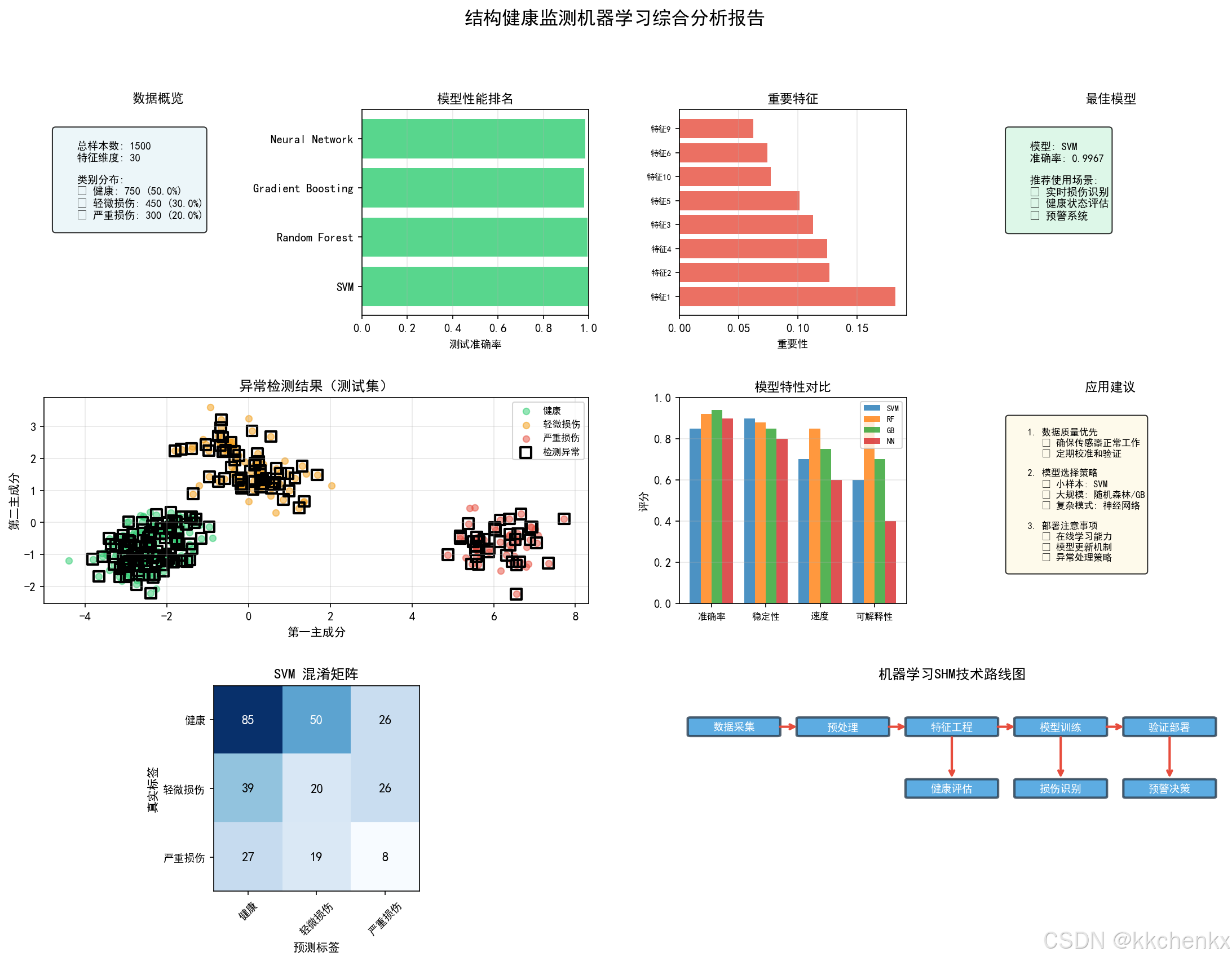
8.2 运行结果

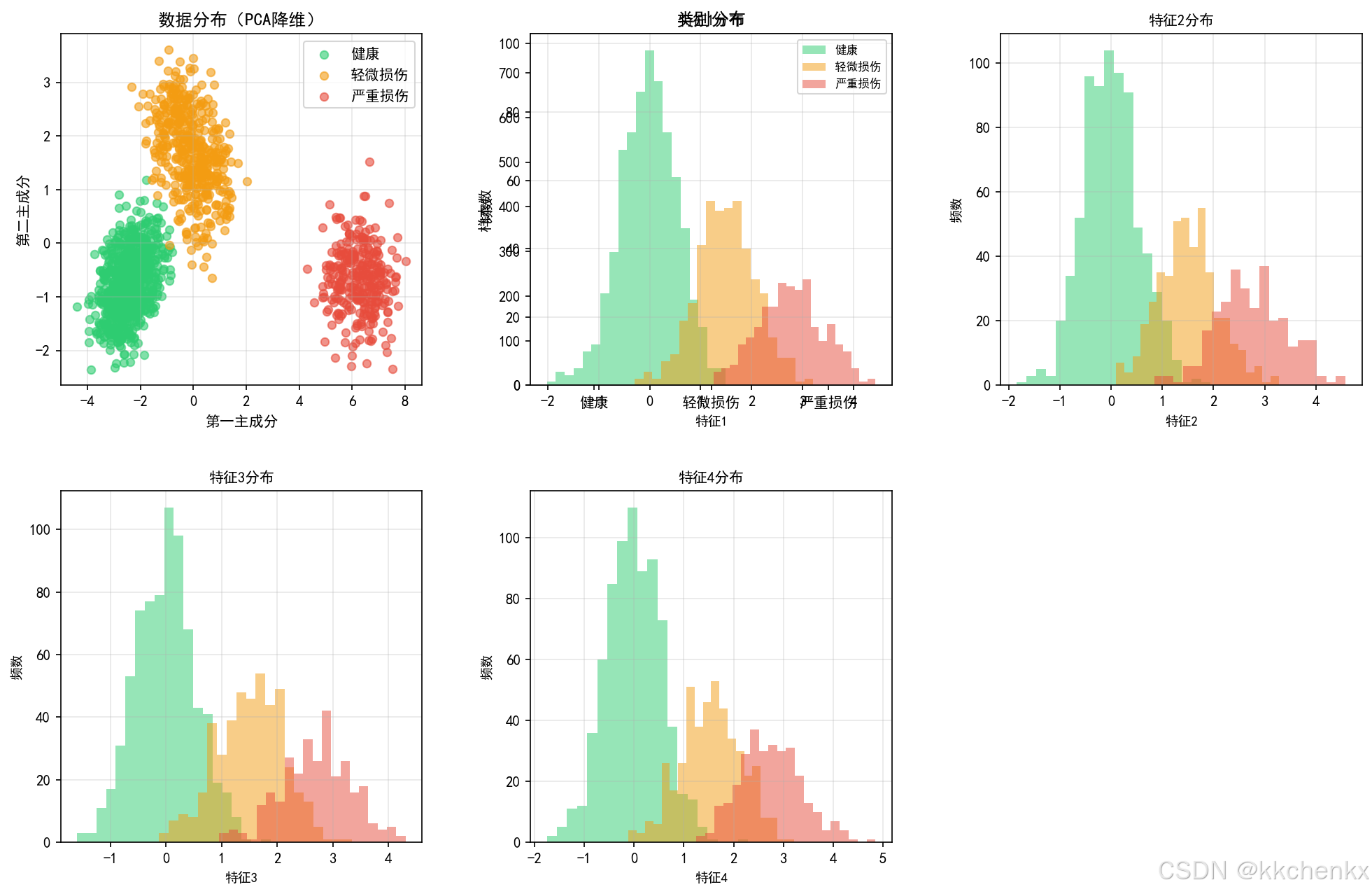
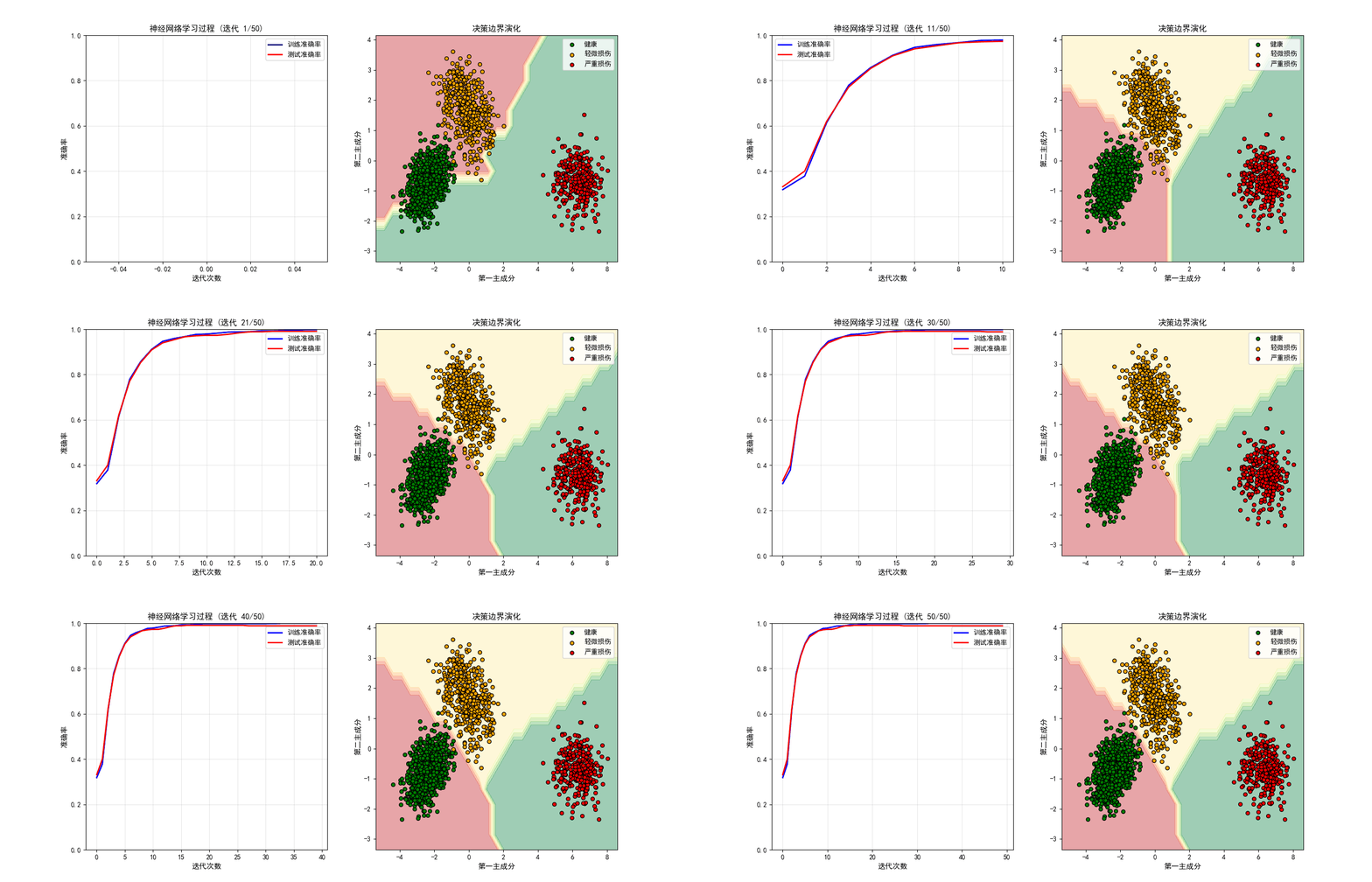
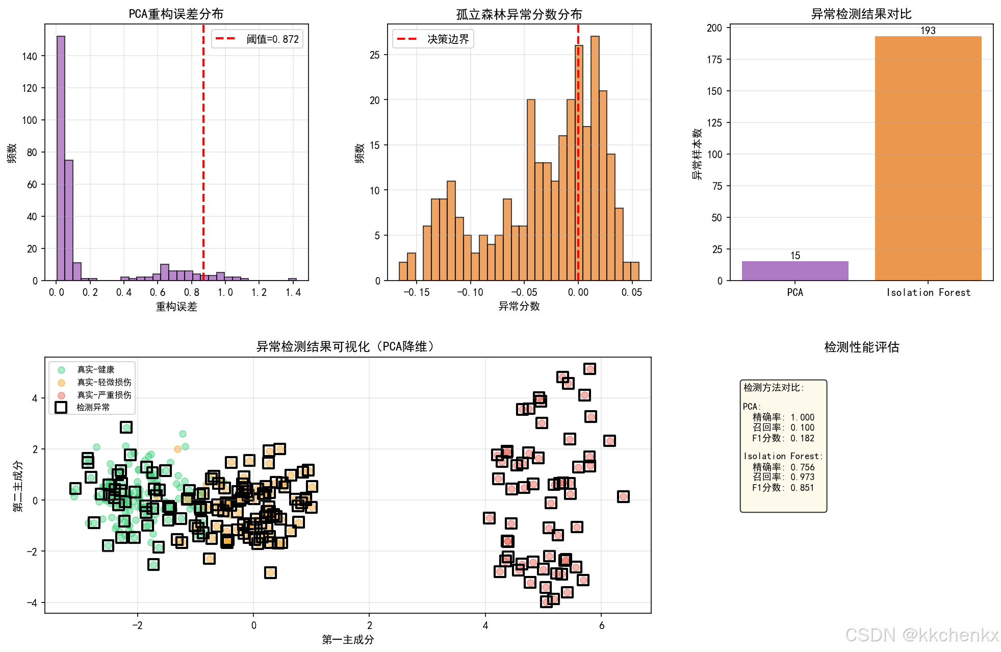
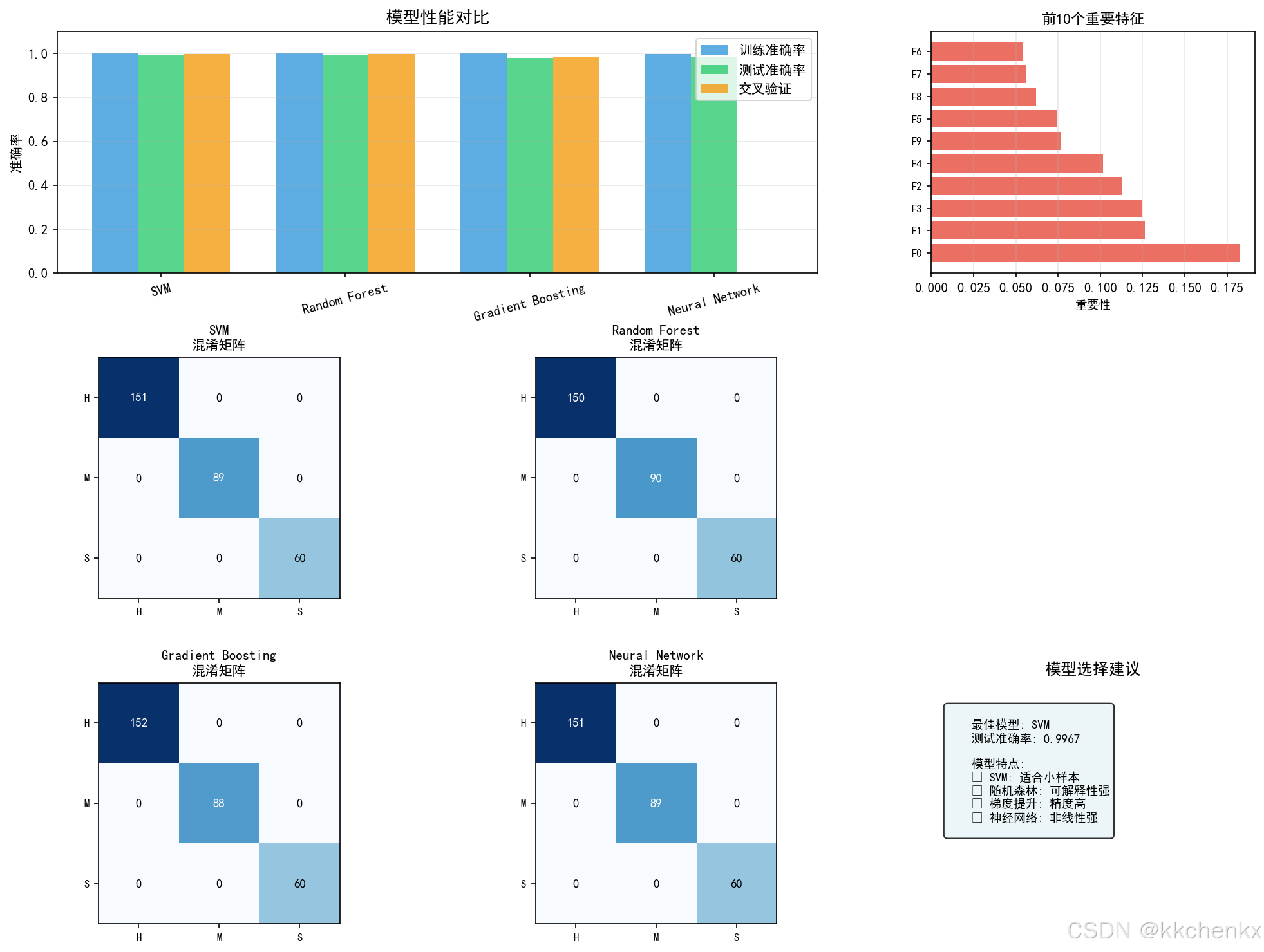
运行上述代码将生成：

数据分布可视化（PCA降维）
模型性能对比图
特征重要性排序
重构误差分布
异常检测结果对比
混淆矩阵

9. 技术挑战与解决方案

9.1 数据不平衡问题

挑战：健康状态数据远多于损伤数据

解决方案：

过采样：SMOTE、ADASYN
欠采样：随机欠采样、Tomek Links
代价敏感学习：调整类别权重
集成方法：BalanceCascade、EasyEnsemble

9.2 标签稀缺问题

挑战：损伤数据难以获取，标签成本高

解决方案：

半监督学习：利用未标记数据
主动学习：选择最有价值的样本进行标注
迁移学习：从相关任务迁移知识
数据增强：通过变换生成新样本

9.3 模型可解释性

挑战：深度学习模型是"黑盒"，难以理解决策依据

解决方案：

SHAP（SHapley Additive exPlanations）
LIME（Local Interpretable Model-agnostic Explanations）
注意力可视化
梯度类激活映射（Grad-CAM）

import shap

def explain_model_with_shap(model, X_train, X_test, feature_names):
    """
    使用SHAP解释模型预测
    
    参数:
    model: 训练好的模型
    X_train: 训练数据
    X_test: 测试数据
    feature_names: 特征名称
    """
    # 创建SHAP解释器
    explainer = shap.TreeExplainer(model)
    shap_values = explainer.shap_values(X_test)
    
    # 可视化
    plt.figure(figsize=(12, 8))
    shap.summary_plot(shap_values, X_test, feature_names=feature_names, show=False)
    plt.title('SHAP特征重要性')
    plt.tight_layout()
    plt.savefig('shap_summary.png', dpi=150)
    plt.close()

9.4 实时性要求

挑战：SHM系统需要实时响应

解决方案：

模型轻量化：剪枝、量化、知识蒸馏
边缘计算：在传感器端进行预处理
增量学习：在线更新模型
硬件加速：GPU、FPGA

附录：Python环境配置

# 创建虚拟环境
conda create -n shm_ml python=3.9

# 激活环境
conda activate shm_ml

# 安装依赖包
pip install numpy scipy scikit-learn matplotlib pandas
pip install tensorflow torch xgboost lightgbm
pip install shap lime

AI Agent技术社区

Agent 垂直技术社区，欢迎活跃、内容共建。

更多推荐

GitHub今日热榜 | 2026-08-06

今日榜单呈现大换血，10个项目中7个为新晋项目。Cloudflare的Agent虚拟环境项目computer空降榜首，提供隔离文件系统和多执行后端支持。腾讯的TencentDB-Agent-Memory虽排名下滑至第3，但日增Star上涨70%。其他亮点包括： loopx为AI Agent团队提供看板管理系统经典面试指南system-design-primer回归榜单 DeepSeek-Reas