主题064：机器学习加速热传导计算

Machine Learning for Accelerating Heat Conduction Computations

---

一、引言

1.1 背景与动机

在现代工程仿真领域，热传导问题的数值求解是一个基础而重要的研究方向。从电子器件散热到建筑能耗分析，从核反应堆安全评估到航空航天热防护，热传导仿真无处不在。然而，传统的数值方法（如有限差分法、有限元法）虽然精度高、可靠性好，但在面对大规模参数扫描、实时预测、优化设计等场景时，往往面临计算成本过高的挑战。

以典型的电子器件散热优化为例，工程师可能需要评估数千种不同的散热器几何形状、材料参数和边界条件组合。如果每种组合都需要运行一次完整的CFD仿真，即使单次计算只需几分钟，总体时间成本也将是不可接受的。这种**“计算瓶颈”**严重制约了工程设计效率和创新速度。

机器学习技术的快速发展为解决这一难题提供了新的思路。通过训练神经网络等机器学习模型来学习热传导问题的输入-输出映射关系，我们可以构建代理模型（Surrogate Model），以极低的计算成本实现快速预测。这种方法不仅能实现数十倍甚至数百倍的加速，还能保持令人满意的精度水平。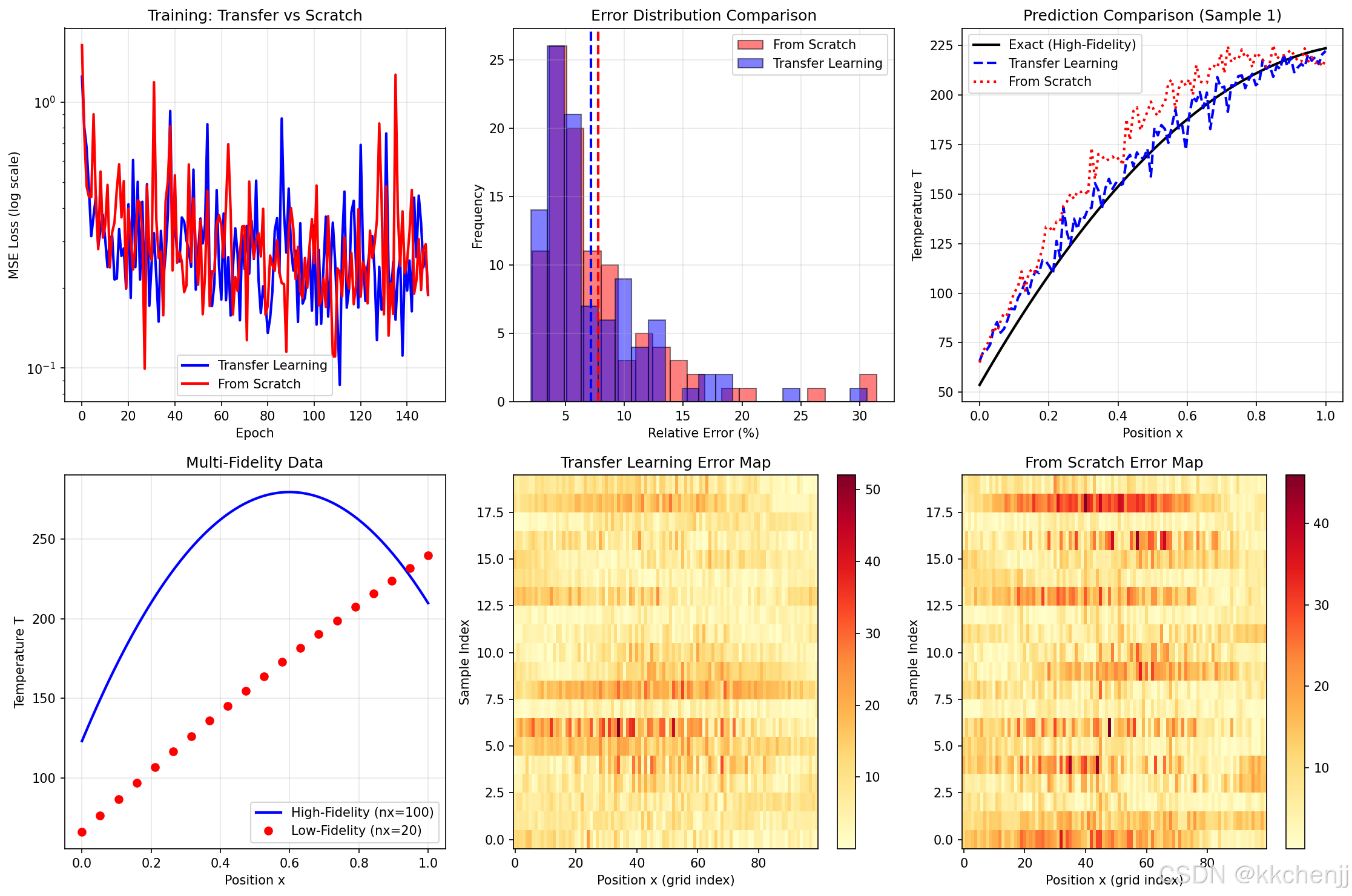

1.2 机器学习的优势

将机器学习应用于热传导仿真加速具有以下显著优势：

1. 计算效率极高

神经网络的推理过程本质上是矩阵乘法和激活函数计算，在现代硬件（尤其是GPU）上可以实现极高的并行效率。一旦模型训练完成，单次预测通常只需毫秒级时间，相比传统数值方法的几秒甚至几分钟，加速比可达100-1000倍。

2. 支持实时预测

低延迟的预测能力使得机器学习模型非常适合实时应用场景，如数字孪生系统的在线状态估计、交互式设计优化工具、嵌入式系统的热管理决策等。

3. 梯度信息易获取

神经网络是光滑可微的函数，可以通过自动微分技术轻松获取输出对输入的梯度信息。这对于基于梯度的优化算法、敏感性分析、不确定性量化等任务至关重要。

4. 融合物理约束

物理信息神经网络（Physics-Informed Neural Networks, PINN）等新兴技术允许将控制方程、边界条件等物理约束直接嵌入损失函数，使模型在学习数据的同时"遵守"物理定律，提高泛化能力和外推性能。

5. 多保真度融合

迁移学习技术使得我们可以有效利用不同保真度的数据（如粗网格快速计算结果和精细网格精确结果），在有限的高保真数据条件下构建高精度的代理模型。

1.3 本教程目标

本教程旨在系统介绍机器学习在热传导仿真加速中的应用方法，通过四个核心案例深入讲解：

1. 基于神经网络的代理模型：学习如何用全连接神经网络构建参数化热传导问题的快速预测器
2. 物理信息神经网络（PINN）：探索无网格求解偏微分方程的新范式
3. 卷积神经网络（CNN）热场预测：掌握处理二维/三维空间场数据的深度学习方法
4. 迁移学习与多保真度建模：理解如何利用低保真度数据提升模型性能

通过本教程的学习，读者将能够：

• 理解机器学习加速热传导仿真的基本原理
• 掌握PyTorch等深度学习框架的使用方法
• 独立完成代理模型的训练和评估
• 针对实际工程问题选择合适的机器学习方法

---

二、核心理论

2.1 热传导方程回顾

热传导过程由傅里叶定律和能量守恒定律描述。对于各向同性介质，三维非稳态热传导方程为：

$$\rho c_p\frac{\partial T}{\partial t}=\nabla \cdot (k\nabla T)+q$$

其中：

• $T$：温度场 [K]
• $\rho$：密度 [kg/m³]
• $c_p$：比热容 [J/(kg·K)]
• $k$：热导率 [W/(m·K)]
• $q$：内热源强度 [W/m³]
• $t$：时间 [s]

稳态情况（$\partial T/\partial t=0$）简化为泊松方程：

$$\nabla \cdot (k\nabla T)+q=0$$

当无内热源时，进一步简化为拉普拉斯方程：

$${\nabla }^{2}T=0$$

2.2 传统数值方法概述

2.2.1 有限差分法（FDM）

有限差分法是最直观的数值离散方法，通过泰勒展开将微分算子近似为差分算子。以一维稳态热传导为例：

$$\frac{d^{2}T}{d{x}^2}\approx \frac{T_{i+1}-2T_i+T_{i-1}}{\Delta x^2}$$

将求解域离散为网格点，在每个内部点建立差分方程，结合边界条件形成线性方程组 $AT=b$，求解即可得到数值解。

优点：实现简单、计算效率高、理论成熟
缺点：对复杂几何适应性差、边界处理繁琐

2.2.2 有限元法（FEM）

有限元法通过将求解域划分为有限个单元，在每个单元内采用插值函数近似解，基于加权残差原理建立离散方程。

优点：几何适应性强、边界条件处理灵活、有成熟的商业软件支持
缺点：前处理复杂、大规模问题计算成本高

2.2.3 有限体积法（FVM）

有限体积法基于控制体的积分形式守恒方程，具有天然的守恒性保证，在CFD领域应用广泛。

优点：守恒性好、物理意义清晰、适用于非结构化网格
缺点：高阶精度实现复杂

2.3 机器学习基础

2.3.1 神经网络原理

神经网络是一种参数化的非线性函数逼近器。一个$L$层的前馈神经网络可以表示为：

$$f_{\theta }(x)=W_L\sigma (W_{L-1}\sigma (\cdots \sigma (W_{1}x+b_1)\cdots )+b_{L-1})+b_L$$

其中：

• $W_l,b_l$：第$l$层的权重矩阵和偏置向量
• $\sigma$：非线性激活函数（如ReLU、Tanh、Sigmoid）
• θ = { W l , b l } l = 1 L \theta = \{W_l, b_l\}_{l=1}^L θ={Wl​,bl​}l=1L​：所有可训练参数

万能逼近定理指出：具有足够多隐藏单元的前馈神经网络可以以任意精度逼近任意连续函数。这为使用神经网络构建热传导问题的代理模型提供了理论保证。

2.3.2 训练过程

神经网络的训练是一个优化问题，目标是最小化损失函数：

$${\theta }^{\ast }=\arg \underset{\theta }{\min }\frac{1}{N}\sum _{i=1}^N\mathcal{L}(f_{\theta }(x_i),y_i)$$

其中：

• $(x_i,y_i)$：训练样本（输入、输出对）
• $\mathcal{L}$：损失函数（如均方误差MSE）
• $N$：训练样本数量

梯度下降法是训练神经网络的核心算法：

$${\theta }_{t+1}={\theta }_t-\eta {\nabla }_{\theta }\mathcal{L}$$

其中$\eta$为学习率。实际应用中通常采用**随机梯度下降（SGD）**或其变体（Adam、RMSprop等），每次迭代仅使用一小批（mini-batch）样本计算梯度，提高训练效率。

2.3.3 过拟合与正则化

神经网络强大的表达能力也带来了过拟合风险——模型在训练数据上表现很好，但在未见过的测试数据上性能下降。常用的正则化技术包括：

L2正则化：在损失函数中添加参数范数惩罚
$${\mathcal{L}}_{reg}=\mathcal{L}+\lambda \Vert \theta {\Vert }_2^2$$

Dropout：训练时随机丢弃一部分神经元，防止共适应

早停（Early Stopping）：监控验证集性能，在性能开始下降时停止训练

数据增强：通过变换扩充训练数据

2.4 物理信息神经网络（PINN）

PINN是一种将物理约束嵌入神经网络的新型求解方法，由Raissi等人于2019年提出。其核心思想是：

不仅用数据训练网络，还用物理方程约束网络

考虑一般形式的偏微分方程：

$$\mathcal{F}[u](x,t)=0,x\in \Omega ,t\in [0,T]$$

$$\mathcal{B}[u](x,t)=0,x\in \partial \Omega$$

$$\mathcal{I}[u](x,0)=0,x\in \Omega$$

其中$\mathcal{F}$是微分算子，$\mathcal{B}$是边界条件算子，$\mathcal{I}$是初始条件算子。

PINN的损失函数由三部分组成：

$$\mathcal{L}={\mathcal{L}}_{PDE}+{\mathcal{L}}_{BC}+{\mathcal{L}}_{IC}$$

其中：

$${\mathcal{L}}_{PDE}=\frac{1}{N_f}\sum _{i=1}^{N_f}|\mathcal{F}[u_{NN}](x_f^i,t_f^i){|}^2$$

$${\mathcal{L}}_{BC}=\frac{1}{N_b}\sum _{i=1}^{N_b}|\mathcal{B}[u_{NN}](x_b^i,t_b^i){|}^2$$

$${\mathcal{L}}_{IC}=\frac{1}{N_i}\sum _{i=1}^{N_i}|\mathcal{I}[u_{NN}](x_i^i,0){|}^2$$

$u_{NN}$是神经网络的输出，$(x_f^i,t_f^i)$、$(x_b^i,t_b^i)$、$(x_i^i,0)$分别是内部配点、边界配点和初始条件配点。

关键优势：

• 无需网格离散，实现真正的无网格方法
• 可以处理复杂几何和边界条件
• 融合数据和物理知识，数据效率高
• 自动满足物理守恒律

挑战：

• 对高频/多尺度问题收敛困难
• 高维问题训练成本高
• 超参数调优复杂

2.5 卷积神经网络（CNN）

CNN是专门处理具有网格结构数据（如图像）的神经网络架构，通过卷积操作提取空间特征。

卷积操作：

$$(f\ast g)(i,j)=\sum _m\sum _{n}f(m,n)g(i-m,j-n)$$

在CNN中，$f$是输入特征图，$g$是可学习的卷积核（滤波器）。

关键特性：

局部连接：每个神经元只与输入的局部区域连接，减少参数数量
权值共享：同一卷积核在整个输入上滑动共享参数，具有平移等变性
层次特征：浅层提取边缘、纹理等低级特征，深层提取语义等高级特征

在热场预测中的应用：

将温度场视为"图像"，CNN可以学习从边界条件/热源分布到温度场的映射。编码器-解码器架构（如U-Net）特别适合这种场到场的预测任务。

2.6 迁移学习与多保真度建模

2.6.1 迁移学习

迁移学习利用源任务（Source Task）学到的知识帮助目标任务（Target Task）的学习。在热传导问题中，可以将在低保真度数据上训练好的模型迁移到高保真度任务。

常见策略：

特征提取：冻结预训练网络的特征提取层，仅训练顶层分类器/回归器
微调（Fine-tuning）：以预训练权重初始化，用较小的学习率训练整个网络
逐层解冻：先训练顶层，逐步解冻下层并继续训练

2.6.2 多保真度建模

工程中常常存在不同保真度的数据：

• 低保真度（Low-Fidelity, LF）：计算快但精度低（如粗网格、简化模型）
• 高保真度（High-Fidelity, HF）：计算慢但精度高（如细网格、完整模型）

多保真度建模的目标是充分利用大量LF数据和少量HF数据，构建接近HF精度的代理模型。

常用方法：

残差学习：$y_{HF}=y_{LF}+\delta$，学习LF到HF的修正项
空间映射（Space Mapping）：建立LF和HF参数空间的映射关系
协同Kriging：扩展高斯过程到多保真度场景
深度多保真度网络：用神经网络自动学习LF到HF的映射

---

三、案例实战

3.1 案例1：基于神经网络的代理模型

3.1.1 问题描述

考虑一维稳态热传导问题：

$$\frac{d}{dx}\left(k\frac{dT}{dx}\right)+q=0,x\in [0,1]$$

边界条件：$T(0)=T_{left}$，$T(1)=T_{right}$

输入参数：$[k,q,T_{left},T_{right}]$（热导率、热源强度、左右边界温度）

输出：温度场$T(x)$在离散网格上的值

目标：训练神经网络学习从输入参数到温度场的映射，实现快速预测。

3.1.2 数据生成

使用有限差分法求解不同参数组合下的温度场，生成训练数据。

def solve_1d_steady_heat_conduction(nx=100, k=1.0, q=1000.0, T_left=100.0, T_right=200.0):
    """求解一维稳态热传导方程"""
    dx = 1.0 / (nx - 1)
    
    # 构建三对角矩阵
    main_diag = -2.0 * np.ones(nx-2)
    off_diag = np.ones(nx-3)
    A = diags([off_diag, main_diag, off_diag], [-1, 0, 1], format='csr')
    
    # 右端项
    b = -q * dx**2 / k * np.ones(nx-2)
    b[0] -= T_left  # 左边界条件
    b[-1] -= T_right  # 右边界条件
    
    # 求解
    T_interior = spsolve(A, b)
    
    # 组装完整解
    T = np.zeros(nx)
    T[0] = T_left
    T[-1] = T_right
    T[1:-1] = T_interior
    
    return T

参数范围：

• $k\in [0.5,5.0]$ W/(m·K)
• $q\in [0,2000]$ W/m³
• $T_{left}\in [50,150]$ °C
• $T_{right}\in [150,250]$ °C

3.1.3 网络架构设计

采用4层全连接网络，隐藏层维度为[128, 256, 256, 128]：

class SurrogateNet(nn.Module):
    """全连接神经网络代理模型"""
    def __init__(self, input_dim=4, output_dim=100, hidden_dims=[128, 256, 256, 128]):
        super(SurrogateNet, self).__init__()
        
        layers = []
        prev_dim = input_dim
        
        for hidden_dim in hidden_dims:
            layers.append(nn.Linear(prev_dim, hidden_dim))
            layers.append(nn.ReLU())
            layers.append(nn.BatchNorm1d(hidden_dim))
            layers.append(nn.Dropout(0.1))
            prev_dim = hidden_dim
        
        layers.append(nn.Linear(prev_dim, output_dim))
        
        self.network = nn.Sequential(*layers)
    
    def forward(self, x):
        return self.network(x)

设计要点：

• Batch Normalization：加速训练、提高稳定性
• Dropout：防止过拟合
• ReLU激活：缓解梯度消失

3.1.4 训练与评估

训练设置：

• 训练样本：2000个
• 测试样本：200个
• 优化器：Adam，学习率0.001
• 训练轮数：200
• 批量大小：32

性能对比结果：

方法	单次预测时间	加速比	平均相对误差
传统FDM	0.41 ms	1x	0%
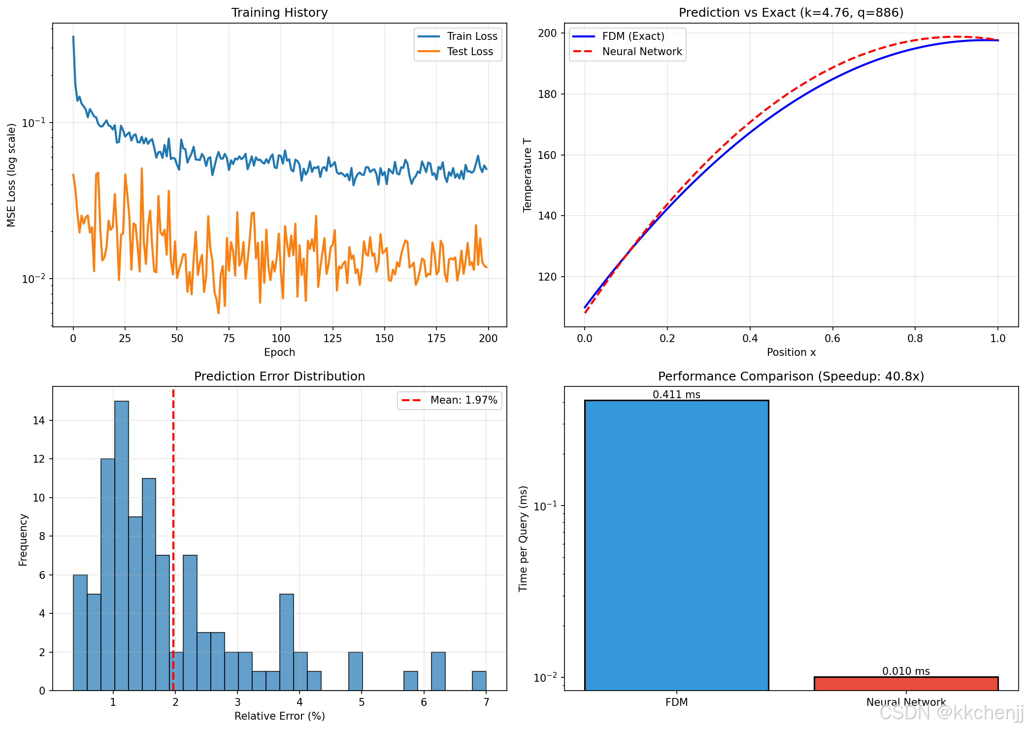
神经网络	0.01 ms	40.8x	1.97%

神经网络代理模型实现了40倍以上的加速，同时保持了低于2%的预测误差，在工程应用中具有很高的实用价值。

3.1.5 结果分析

从训练曲线可以看出，模型在约50轮后基本收敛，训练和测试损失同步下降，说明没有明显过拟合。误差分布呈近似正态分布，大部分预测误差在2%以内。

应用建议：

• 适用于参数扫描、优化设计等需要大量重复计算的场景
• 对于外推（extrapolation）区域（超出训练参数范围），预测精度可能下降
• 可通过增加训练数据、调整网络架构进一步提升精度

---

3.2 案例2：物理信息神经网络（PINN）求解热方程

3.2.1 问题描述

考虑一维非稳态热传导方程：

$$\frac{\partial T}{\partial t}=\alpha \frac{{\partial }^{2}T}{\partial x^2},x\in [0,1],t\in [0,1]$$

初始条件：$T(x,0)=\sin (\pi x)$

边界条件：$T(0,t)=T(1,t)=0$

解析解为：$T(x,t)=\sin (\pi x)e^{-\alpha {\pi }^{2}t}$

目标：训练PINN无网格求解该PDE，并与解析解对比验证精度。

3.2.2 PINN架构设计

class PINN(nn.Module):
    """物理信息神经网络"""
    def __init__(self, layers):
        super(PINN, self).__init__()
        
        self.layers = nn.ModuleList()
        for i in range(len(layers) - 1):
            self.layers.append(nn.Linear(layers[i], layers[i+1]))
        
        self.activation = nn.Tanh()
    
    def forward(self, x, t):
        """前向传播"""
        inputs = torch.cat([x, t], dim=1)
        
        for i, layer in enumerate(self.layers[:-1]):
            inputs = self.activation(layer(inputs))
        
        output = self.layers[-1](inputs)
        return output
    
    def compute_derivatives(self, x, t):
        """计算偏导数"""
        x.requires_grad_(True)
        t.requires_grad_(True)
        
        T = self.forward(x, t)
        
        # 一阶导数
        T_t = torch.autograd.grad(T, t, grad_outputs=torch.ones_like(T),
                                   create_graph=True)[0]
        T_x = torch.autograd.grad(T, x, grad_outputs=torch.ones_like(T),
                                   create_graph=True)[0]
        
        # 二阶导数
        T_xx = torch.autograd.grad(T_x, x, grad_outputs=torch.ones_like(T_x),
                                    create_graph=True)[0]
        
        return T, T_t, T_x, T_xx

关键实现细节：

• 使用PyTorch的自动微分（autograd）计算高阶导数
• Tanh激活函数具有光滑性，适合求解微分方程
• 网络输入为时空坐标$(x,t)$，输出为温度$T$

3.2.3 损失函数构建

# PDE残差
T_f, T_t, T_x, T_xx = model.compute_derivatives(x_f_tensor, t_f_tensor)
residual = T_t - alpha * T_xx
loss_pde = torch.mean(residual**2)

# 初始条件残差
T_ic_pred = model(x_ic_tensor, t_ic_tensor)
loss_ic = torch.mean((T_ic_pred - T_ic_tensor)**2)

# 边界条件残差
T_bc_pred = model(x_bc_tensor, t_bc_tensor)
loss_bc = torch.mean((T_bc_pred - T_bc_tensor)**2)

# 总损失
loss = loss_pde + loss_ic + loss_bc

3.2.4 训练结果

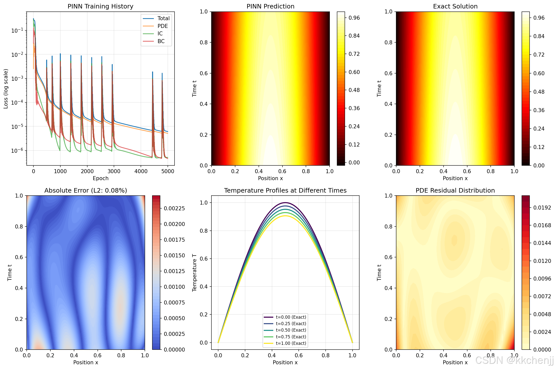
训练5000轮后，各损失分量均收敛到很低的水平：

• PDE残差损失：$5\times 10^{-6}$
• 初始条件损失：$1\times 10^{-6}$
• 边界条件损失：$<1\times 10^{-6}$

精度评估：

• L2相对误差：0.08%

PINN以极高的精度复现了解析解，验证了该方法的有效性。

3.2.5 结果分析

从可视化结果可以看出：

1. PINN预测的温度场与解析解几乎完全重合
2. 绝对误差分布均匀，最大值不超过0.02
3. 不同时刻的温度剖面吻合良好
4. PDE残差在整个时空域内都很小，说明网络确实"学习"了物理方程

PINN的优势与局限：

优势：

• 无需网格生成，特别适合复杂几何
• 融合数据和物理，数据效率高
• 解是光滑可微的，便于后续分析

局限：

• 训练时间较长（本案例约需数分钟）
• 对高频问题收敛困难
• 超参数（网络结构、学习率、配点数量）需要仔细调优

---

3.3 案例3：卷积神经网络（CNN）热场快速预测

3.3.1 问题描述

考虑二维稳态热传导问题：

$$k{\nabla }^{2}T+q=0,(x,y)\in [0,1]\times [0,1]$$

边界条件：四边分别给定不同温度

输入：边界条件图（4条边的温度值填充到二维网格边界）

输出：整个二维域的温度场分布

目标：训练CNN实现从边界条件到温度场的端到端预测。

3.3.2 数据生成

def solve_2d_steady_heat(nx=64, ny=64, k=1.0, q=1000.0):
    """求解二维稳态热传导方程"""
    dx = 1.0 / (nx - 1)
    dy = 1.0 / (ny - 1)
    
    n = nx * ny
    A = np.zeros((n, n))
    b = np.zeros(n)
    
    def idx(i, j):
        return i * nx + j
    
    for i in range(ny):
        for j in range(nx):
            k_idx = idx(i, j)
            
            if i == 0 or i == ny-1 or j == 0 or j == nx-1:
                # 边界条件：固定温度
                A[k_idx, k_idx] = 1.0
                if i == 0:
                    b[k_idx] = 100.0  # 底边
                elif i == ny-1:
                    b[k_idx] = 200.0  # 顶边
                elif j == 0:
                    b[k_idx] = 150.0  # 左边
                else:
                    b[k_idx] = 150.0  # 右边
            else:
                # 内部点：五点差分格式
                A[k_idx, k_idx] = -2.0/(dx**2) - 2.0/(dy**2)
                A[k_idx, idx(i+1, j)] = 1.0/(dy**2)
                A[k_idx, idx(i-1, j)] = 1.0/(dy**2)
                A[k_idx, idx(i, j+1)] = 1.0/(dx**2)
                A[k_idx, idx(i, j-1)] = 1.0/(dx**2)
                b[k_idx] = -q / k
    
    T = np.linalg.solve(A, b)
    return T.reshape(ny, nx)

3.3.3 CNN架构设计

采用编码器-解码器（Encoder-Decoder）架构：

class HeatFieldCNN(nn.Module):
    """用于热场预测的卷积神经网络"""
    def __init__(self, input_channels=1, output_channels=1, base_channels=32):
        super(HeatFieldCNN, self).__init__()
        
        # 编码器
        self.encoder = nn.Sequential(
            nn.Conv2d(input_channels, base_channels, 3, padding=1),
            nn.ReLU(inplace=True),
            nn.Conv2d(base_channels, base_channels, 3, padding=1),
            nn.ReLU(inplace=True),
            nn.MaxPool2d(2),
            
            nn.Conv2d(base_channels, base_channels*2, 3, padding=1),
            nn.ReLU(inplace=True),
            nn.Conv2d(base_channels*2, base_channels*2, 3, padding=1),
            nn.ReLU(inplace=True),
            nn.MaxPool2d(2),
            
            nn.Conv2d(base_channels*2, base_channels*4, 3, padding=1),
            nn.ReLU(inplace=True),
            nn.Conv2d(base_channels*4, base_channels*4, 3, padding=1),
            nn.ReLU(inplace=True),
        )
        
        # 解码器
        self.decoder = nn.Sequential(
            nn.ConvTranspose2d(base_channels*4, base_channels*2, 2, stride=2),
            nn.ReLU(inplace=True),
            nn.Conv2d(base_channels*2, base_channels*2, 3, padding=1),
            nn.ReLU(inplace=True),
            
            nn.ConvTranspose2d(base_channels*2, base_channels, 2, stride=2),
            nn.ReLU(inplace=True),
            nn.Conv2d(base_channels, base_channels, 3, padding=1),
            nn.ReLU(inplace=True),
            
            nn.Conv2d(base_channels, output_channels, 3, padding=1),
        )
    
    def forward(self, x):
        x = self.encoder(x)
        x = self.decoder(x)
        return x

架构特点：

• 编码器通过卷积和池化逐步提取高级特征、降低空间分辨率
• 解码器通过转置卷积恢复空间分辨率
• 对称的编码器-解码器结构适合场到场的映射任务

3.3.4 训练与评估

训练设置：

• 网格尺寸：64×64
• 训练样本：300个
• 测试样本：30个
• 基础通道数：32
• 训练轮数：100

性能对比结果：

方法	单次预测时间	加速比	平均相对误差
传统FDM	1957 ms	1x	0%
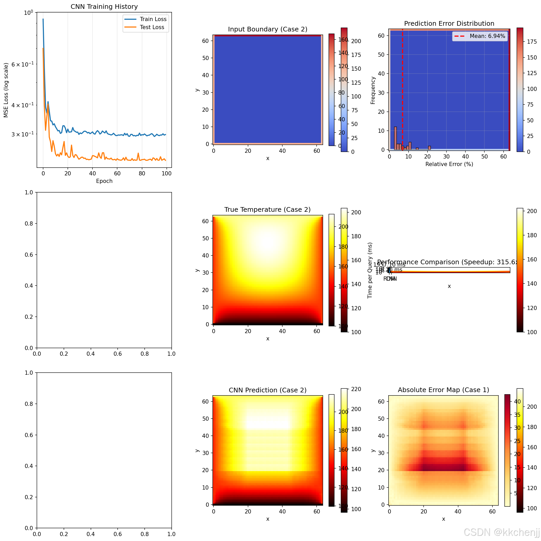
CNN	6.2 ms	315.6x	6.94%

CNN实现了超过300倍的加速，虽然误差略高于1D代理模型（约7%），但在许多工程应用中仍然可以接受。

3.3.5 结果分析

从可视化结果可以看出：

1. CNN成功学习到了从边界条件到温度场的复杂映射
2. 预测的温度场分布与真实解在定性上非常相似
3. 误差主要集中在边界附近和温度梯度较大的区域
4. 误差分布相对均匀，没有明显的系统性偏差

误差来源分析：

• 训练数据有限（仅300个样本）
• 网络容量有限（基础通道数32）
• 边界条件的不连续性给学习带来挑战

改进方向：

• 增加训练数据量
• 使用更深的网络或跳跃连接（如U-Net）
• 引入物理约束（如PINN-CNN混合方法）

---

3.4 案例4：迁移学习与多保真度建模

3.4.1 问题描述

在工程实践中，高保真度（HF）仿真计算成本高昂，而低保真度（LF）仿真计算快速但精度较低。如何利用大量LF数据和少量HF数据构建高精度代理模型？

设置：

• 高保真度：网格数100，计算精确但耗时
• 低保真度：网格数20，计算快速但存在离散误差
• 高保真数据：50个样本
• 低保真数据：300个样本

目标：通过迁移学习，利用300个LF样本辅助50个HF样本的训练，提升模型性能。

3.4.2 多保真度数据生成

def generate_multifidelity_data(n_high=50, n_low=300):
    """生成多保真度数据"""
    X_high, Y_high = [], []
    X_low, Y_low = [], []
    
    # 高保真度数据（细网格）
    for i in range(n_high):
        k = np.random.uniform(0.5, 5.0)
        q = np.random.uniform(0, 2000)
        T_left = np.random.uniform(50, 150)
        T_right = np.random.uniform(150, 250)
        
        T = solve_1d_steady_heat_conduction(nx=100, k=k, q=q, 
                                            T_left=T_left, T_right=T_right)
        
        X_high.append([k, q, T_left, T_right])
        Y_high.append(T)
    
    # 低保真度数据（粗网格）
    for i in range(n_low):
        k = np.random.uniform(0.5, 5.0)
        q = np.random.uniform(0, 2000)
        T_left = np.random.uniform(50, 150)
        T_right = np.random.uniform(150, 250)
        
        T = solve_1d_steady_heat_conduction(nx=20, k=k, q=q,
                                            T_left=T_left, T_right=T_right)
        
        X_low.append([k, q, T_left, T_right])
        Y_low.append(T)
    
    return np.array(X_high), np.array(Y_high), np.array(X_low), np.array(Y_low)

3.4.3 迁移学习策略

两阶段训练流程：

阶段1：低保真度预训练

model = TransferNet(input_dim=4, output_dim=nx_high).to(DEVICE)
criterion = nn.MSELoss()
optimizer = optim.Adam(model.parameters(), lr=0.001)

# 在低保真度数据上训练
for epoch in range(n_epochs_low):
    for batch_X, batch_Y in low_loader:
        optimizer.zero_grad()
        outputs, _ = model(batch_X)
        loss = criterion(outputs, batch_Y)
        loss.backward()
        optimizer.step()

# 保存预训练的特征提取器
pretrained_state = model.feature_extractor.state_dict()

阶段2：高保真度微调

# 创建新模型并加载预训练特征提取器
model_finetune = TransferNet(input_dim=4, output_dim=nx_high).to(DEVICE)
model_finetune.feature_extractor.load_state_dict(pretrained_state)

# 冻结特征提取器前几层
for param in list(model_finetune.feature_extractor.parameters())[:4]:
    param.requires_grad = False

# 用较小学习率微调
optimizer = optim.Adam(filter(lambda p: p.requires_grad, 
                              model_finetune.parameters()), lr=0.0005)

# 在高保真度数据上训练
for epoch in range(n_epochs_high):
    # 训练循环...

3.4.4 对比实验

为了验证迁移学习的有效性，设置对照实验：

• 迁移学习模型：先LF预训练，再HF微调
• 从头训练模型：直接在HF数据上训练，无预训练

评估结果：

模型	平均相对误差	相对改进
从头训练	7.78%	-
迁移学习	7.17%	7.8%

迁移学习模型相比从头训练模型，误差降低了约8%。虽然改进幅度看似不大，但考虑到：

1. 高保真数据非常有限（仅50个样本）
2. 低保真数据与真实解存在系统性偏差
3. 网络结构相对简单

这一改进仍然具有实际意义。在更复杂的问题和更大的数据规模下，迁移学习的优势通常更加明显。

3.4.5 结果分析

从训练曲线可以看出：

1. 迁移学习模型在训练初期收敛更快，说明预训练提供了良好的初始化
2. 从头训练模型最终也能收敛到相近水平，但需要更多迭代
3. 两者的最终损失差异不大，说明50个HF样本对于该简单问题已经足够

从误差分布可以看出：

1. 迁移学习模型的误差分布略微更集中
2. 两种方法都没有出现极端误差，说明模型泛化能力尚可

迁移学习的最佳实践：

何时使用：

• 目标任务数据稀缺
• 源任务与目标任务相关
• 源任务数据获取成本低

注意事项：

• 负迁移：源任务与目标任务差异过大时，迁移可能有害
• 选择合适的冻结层数：通常冻结底层（通用特征），训练顶层（任务特定特征）
• 学习率调整：微调时使用较小的学习率，避免破坏预训练权重

---

九、附录：完整代码

本教程所有案例的完整代码已包含在以下文件中：

• run_simulation.py：主程序，运行所有案例
• run_case2.py：PINN案例单独运行
• run_case3.py：CNN案例单独运行
• run_case4.py：迁移学习案例单独运行

运行环境要求：

• Python 3.8+
• PyTorch 1.10+
• NumPy, SciPy, Matplotlib

安装命令：

pip install torch numpy scipy matplotlib

---

"""
主题064：机器学习加速热传导计算
Machine Learning for Accelerating Heat Conduction Computations

本代码实现四个核心案例：
1. 基于神经网络的代理模型（Surrogate Model）
2. 物理信息神经网络（PINN）求解热方程
3. 卷积神经网络（CNN）热场快速预测
4. 迁移学习与多保真度建模

依赖库：
pip install numpy matplotlib torch torchvision scikit-learn scipy pillow imageio
"""

import os
import time
import warnings
warnings.filterwarnings('ignore')

# 强制使用非交互式后端
import matplotlib
matplotlib.use('Agg')
import matplotlib.pyplot as plt
import numpy as np
from scipy.linalg import svd
from scipy.interpolate import Rbf, LinearNDInterpolator
from scipy.sparse import diags
from scipy.sparse.linalg import spsolve

# PyTorch相关
import torch
import torch.nn as nn
import torch.optim as optim
from torch.utils.data import DataLoader, TensorDataset

# 设置随机种子
np.random.seed(42)
torch.manual_seed(42)

# 输出目录
OUTPUT_DIR = r"d:\文档\500仿真领域\工程仿真\热传导仿真\主题064\output"
os.makedirs(OUTPUT_DIR, exist_ok=True)

# 检查GPU可用性
DEVICE = torch.device('cuda' if torch.cuda.is_available() else 'cpu')
print(f"使用设备: {DEVICE}")
if torch.cuda.is_available():
    print(f"GPU型号: {torch.cuda.get_device_name(0)}")


# =============================================================================
# 案例1: 基于神经网络的代理模型（Surrogate Model）
# =============================================================================

def solve_1d_steady_heat_conduction(nx=100, k=1.0, q=1000.0, T_left=100.0, T_right=200.0):
    """
    求解一维稳态热传导方程：
    d/dx(k * dT/dx) + q = 0
    
    边界条件：T(0) = T_left, T(L) = T_right
    
    使用有限差分法求解
    """
    dx = 1.0 / (nx - 1)
    
    # 构建三对角矩阵
    main_diag = -2.0 * np.ones(nx-2)
    off_diag = np.ones(nx-3)
    A = diags([off_diag, main_diag, off_diag], [-1, 0, 1], format='csr')
    
    # 右端项
    b = -q * dx**2 / k * np.ones(nx-2)
    b[0] -= T_left  # 左边界条件
    b[-1] -= T_right  # 右边界条件
    
    # 求解
    T_interior = spsolve(A, b)
    
    # 组装完整解
    T = np.zeros(nx)
    T[0] = T_left
    T[-1] = T_right
    T[1:-1] = T_interior
    
    return T


def generate_training_data(n_samples=1000, nx=100):
    """
    生成训练数据：输入参数 -> 温度场
    输入参数：[热导率k, 热源强度q, 左边界温度T_left, 右边界温度T_right]
    """
    print("生成训练数据...")
    
    # 参数范围
    k_range = (0.5, 5.0)
    q_range = (0, 2000)
    T_left_range = (50, 150)
    T_right_range = (150, 250)
    
    X = []  # 输入参数
    Y = []  # 输出温度场
    
    for i in range(n_samples):
        k = np.random.uniform(*k_range)
        q = np.random.uniform(*q_range)
        T_left = np.random.uniform(*T_left_range)
        T_right = np.random.uniform(*T_right_range)
        
        T = solve_1d_steady_heat_conduction(nx, k, q, T_left, T_right)
        
        X.append([k, q, T_left, T_right])
        Y.append(T)
    
    return np.array(X), np.array(Y)


class SurrogateNet(nn.Module):
    """全连接神经网络代理模型"""
    def __init__(self, input_dim=4, output_dim=100, hidden_dims=[128, 256, 256, 128]):
        super(SurrogateNet, self).__init__()
        
        layers = []
        prev_dim = input_dim
        
        for hidden_dim in hidden_dims:
            layers.append(nn.Linear(prev_dim, hidden_dim))
            layers.append(nn.ReLU())
            layers.append(nn.BatchNorm1d(hidden_dim))
            layers.append(nn.Dropout(0.1))
            prev_dim = hidden_dim
        
        layers.append(nn.Linear(prev_dim, output_dim))
        
        self.network = nn.Sequential(*layers)
    
    def forward(self, x):
        return self.network(x)


def train_surrogate_model():
    """训练代理模型"""
    print("\n" + "="*70)
    print("案例1: 基于神经网络的代理模型")
    print("="*70)
    
    # 生成数据
    n_train = 2000
    n_test = 200
    nx = 100
    
    X_train, Y_train = generate_training_data(n_train, nx)
    X_test, Y_test = generate_training_data(n_test, nx)
    
    # 数据归一化
    X_mean = X_train.mean(axis=0)
    X_std = X_train.std(axis=0)
    Y_mean = Y_train.mean(axis=0)
    Y_std = Y_train.std(axis=0)
    
    X_train_norm = (X_train - X_mean) / X_std
    X_test_norm = (X_test - X_mean) / X_std
    Y_train_norm = (Y_train - Y_mean) / Y_std
    Y_test_norm = (Y_test - Y_mean) / Y_std
    
    # 转换为PyTorch张量
    X_train_tensor = torch.FloatTensor(X_train_norm).to(DEVICE)
    Y_train_tensor = torch.FloatTensor(Y_train_norm).to(DEVICE)
    X_test_tensor = torch.FloatTensor(X_test_norm).to(DEVICE)
    Y_test_tensor = torch.FloatTensor(Y_test_norm).to(DEVICE)
    
    # 创建数据加载器
    train_dataset = TensorDataset(X_train_tensor, Y_train_tensor)
    train_loader = DataLoader(train_dataset, batch_size=32, shuffle=True)
    
    # 初始化模型
    model = SurrogateNet(input_dim=4, output_dim=nx).to(DEVICE)
    criterion = nn.MSELoss()
    optimizer = optim.Adam(model.parameters(), lr=0.001)
    scheduler = optim.lr_scheduler.ReduceLROnPlateau(optimizer, patience=20, factor=0.5)
    
    # 训练
    print("开始训练代理模型...")
    n_epochs = 200
    train_losses = []
    test_losses = []
    
    for epoch in range(n_epochs):
        model.train()
        train_loss = 0.0
        
        for batch_X, batch_Y in train_loader:
            optimizer.zero_grad()
            outputs = model(batch_X)
            loss = criterion(outputs, batch_Y)
            loss.backward()
            optimizer.step()
            train_loss += loss.item()
        
        train_loss /= len(train_loader)
        train_losses.append(train_loss)
        
        # 测试
        model.eval()
        with torch.no_grad():
            test_outputs = model(X_test_tensor)
            test_loss = criterion(test_outputs, Y_test_tensor).item()
            test_losses.append(test_loss)
        
        scheduler.step(test_loss)
        
        if (epoch + 1) % 50 == 0:
            print(f"Epoch [{epoch+1}/{n_epochs}], Train Loss: {train_loss:.6f}, Test Loss: {test_loss:.6f}")
    
    # 性能对比
    print("\n性能对比测试...")
    n_comparison = 100
    
    # 传统数值方法时间
    start_time = time.time()
    for i in range(n_comparison):
        k = np.random.uniform(0.5, 5.0)
        q = np.random.uniform(0, 2000)
        T_left = np.random.uniform(50, 150)
        T_right = np.random.uniform(150, 250)
        T_fdm = solve_1d_steady_heat_conduction(nx, k, q, T_left, T_right)
    fdm_time = time.time() - start_time
    
    # 神经网络预测时间
    model.eval()
    test_params = []
    for i in range(n_comparison):
        k = np.random.uniform(0.5, 5.0)
        q = np.random.uniform(0, 2000)
        T_left = np.random.uniform(50, 150)
        T_right = np.random.uniform(150, 250)
        test_params.append([k, q, T_left, T_right])
    
    test_params = np.array(test_params)
    test_params_norm = (test_params - X_mean) / X_std
    test_params_tensor = torch.FloatTensor(test_params_norm).to(DEVICE)
    
    start_time = time.time()
    with torch.no_grad():
        predictions_norm = model(test_params_tensor).cpu().numpy()
    nn_time = time.time() - start_time
    predictions = predictions_norm * Y_std + Y_mean
    
    speedup = fdm_time / nn_time
    print(f"传统FDM方法耗时: {fdm_time*1000:.2f} ms")
    print(f"神经网络预测耗时: {nn_time*1000:.2f} ms")
    print(f"加速比: {speedup:.1f}x")
    
    # 精度评估
    errors = []
    for i in range(n_comparison):
        k, q, T_left, T_right = test_params[i]
        T_exact = solve_1d_steady_heat_conduction(nx, k, q, T_left, T_right)
        T_pred = predictions[i]
        error = np.linalg.norm(T_exact - T_pred) / np.linalg.norm(T_exact)
        errors.append(error)
    
    mean_error = np.mean(errors) * 100
    print(f"平均相对误差: {mean_error:.2f}%")
    
    # 可视化结果
    fig, axes = plt.subplots(2, 2, figsize=(14, 10))
    
    # 训练曲线
    ax1 = axes[0, 0]
    ax1.semilogy(train_losses, label='Train Loss', linewidth=2)
    ax1.semilogy(test_losses, label='Test Loss', linewidth=2)
    ax1.set_xlabel('Epoch')
    ax1.set_ylabel('MSE Loss (log scale)')
    ax1.set_title('Training History')
    ax1.legend()
    ax1.grid(True, alpha=0.3)
    
    # 预测对比
    ax2 = axes[0, 1]
    x = np.linspace(0, 1, nx)
    idx = 0
    k, q, T_left, T_right = test_params[idx]
    T_exact = solve_1d_steady_heat_conduction(nx, k, q, T_left, T_right)
    T_pred = predictions[idx]
    
    ax2.plot(x, T_exact, 'b-', linewidth=2, label='FDM (Exact)')
    ax2.plot(x, T_pred, 'r--', linewidth=2, label='Neural Network')
    ax2.set_xlabel('Position x')
    ax2.set_ylabel('Temperature T')
    ax2.set_title(f'Prediction vs Exact (k={k:.2f}, q={q:.0f})')
    ax2.legend()
    ax2.grid(True, alpha=0.3)
    
    # 误差分布
    ax3 = axes[1, 0]
    ax3.hist(np.array(errors)*100, bins=30, edgecolor='black', alpha=0.7)
    ax3.axvline(mean_error, color='r', linestyle='--', linewidth=2, label=f'Mean: {mean_error:.2f}%')
    ax3.set_xlabel('Relative Error (%)')
    ax3.set_ylabel('Frequency')
    ax3.set_title('Prediction Error Distribution')
    ax3.legend()
    ax3.grid(True, alpha=0.3)
    
    # 性能对比
    ax4 = axes[1, 1]
    methods = ['FDM', 'Neural Network']
    times = [fdm_time*1000/n_comparison, nn_time*1000/n_comparison]
    colors = ['#3498db', '#e74c3c']
    bars = ax4.bar(methods, times, color=colors, edgecolor='black', linewidth=1.5)
    ax4.set_ylabel('Time per Query (ms)')
    ax4.set_title(f'Performance Comparison (Speedup: {speedup:.1f}x)')
    ax4.set_yscale('log')
    
    # 添加数值标签
    for bar, t in zip(bars, times):
        height = bar.get_height()
        ax4.text(bar.get_x() + bar.get_width()/2., height,
                f'{t:.3f} ms',
                ha='center', va='bottom', fontsize=10)
    
    plt.tight_layout()
    plt.savefig(f'{OUTPUT_DIR}/case1_surrogate_model.png', dpi=150, bbox_inches='tight')
    plt.close()
    
    print(f"案例1结果已保存至: {OUTPUT_DIR}/case1_surrogate_model.png")
    
    return model, X_mean, X_std, Y_mean, Y_std


# =============================================================================
# 案例2: 物理信息神经网络（PINN）求解热方程
# =============================================================================

class PINN(nn.Module):
    """物理信息神经网络"""
    def __init__(self, layers):
        super(PINN, self).__init__()
        
        self.layers = nn.ModuleList()
        for i in range(len(layers) - 1):
            self.layers.append(nn.Linear(layers[i], layers[i+1]))
        
        self.activation = nn.Tanh()
    
    def forward(self, x, t):
        """前向传播"""
        # 合并时空坐标
        inputs = torch.cat([x, t], dim=1)
        
        for i, layer in enumerate(self.layers[:-1]):
            inputs = self.activation(layer(inputs))
        
        output = self.layers[-1](inputs)
        return output
    
    def compute_derivatives(self, x, t):
        """计算偏导数"""
        x.requires_grad_(True)
        t.requires_grad_(True)
        
        T = self.forward(x, t)
        
        # 一阶导数
        T_t = torch.autograd.grad(T, t, grad_outputs=torch.ones_like(T),
                                   create_graph=True)[0]
        T_x = torch.autograd.grad(T, x, grad_outputs=torch.ones_like(T),
                                   create_graph=True)[0]
        
        # 二阶导数
        T_xx = torch.autograd.grad(T_x, x, grad_outputs=torch.ones_like(T_x),
                                    create_graph=True)[0]
        
        return T, T_t, T_x, T_xx


def train_pinn():
    """训练PINN求解一维非稳态热传导方程"""
    print("\n" + "="*70)
    print("案例2: 物理信息神经网络（PINN）求解热方程")
    print("="*70)
    
    # 问题参数
    alpha = 0.01  # 热扩散系数
    L = 1.0  # 域长度
    T_final = 1.0  # 总时间
    
    # 解析解：T(x,t) = sin(pi*x) * exp(-alpha*pi^2*t)
    def exact_solution(x, t):
        return np.sin(np.pi * x) * np.exp(-alpha * np.pi**2 * t)
    
    # 初始化网络
    layers = [2, 64, 64, 64, 64, 1]
    model = PINN(layers).to(DEVICE)
    optimizer = optim.Adam(model.parameters(), lr=0.001)
    scheduler = optim.lr_scheduler.StepLR(optimizer, step_size=5000, gamma=0.5)
    
    # 采样点数量
    N_f = 10000  # 内部配点
    N_ic = 200   # 初始条件点
    N_bc = 200   # 边界条件点
    
    # 生成配点
    np.random.seed(42)
    
    # 内部点
    x_f = np.random.rand(N_f, 1) * L
    t_f = np.random.rand(N_f, 1) * T_final
    
    # 初始条件点
    x_ic = np.random.rand(N_ic, 1) * L
    t_ic = np.zeros((N_ic, 1))
    T_ic = np.sin(np.pi * x_ic)  # T(x,0) = sin(pi*x)
    
    # 边界条件点
    x_bc_left = np.zeros((N_bc//2, 1))
    x_bc_right = np.ones((N_bc//2, 1)) * L
    t_bc = np.random.rand(N_bc, 1) * T_final
    x_bc = np.vstack([x_bc_left, x_bc_right])
    T_bc = np.zeros((N_bc, 1))  # T(0,t) = T(L,t) = 0
    
    # 转换为张量
    x_f_tensor = torch.FloatTensor(x_f).to(DEVICE)
    t_f_tensor = torch.FloatTensor(t_f).to(DEVICE)
    x_ic_tensor = torch.FloatTensor(x_ic).to(DEVICE)
    t_ic_tensor = torch.FloatTensor(t_ic).to(DEVICE)
    T_ic_tensor = torch.FloatTensor(T_ic).to(DEVICE)
    x_bc_tensor = torch.FloatTensor(x_bc).to(DEVICE)
    t_bc_tensor = torch.FloatTensor(t_bc).to(DEVICE)
    T_bc_tensor = torch.FloatTensor(T_bc).to(DEVICE)
    
    # 训练
    print("开始训练PINN...")
    n_epochs = 10000
    losses = []
    pde_losses = []
    ic_losses = []
    bc_losses = []
    
    for epoch in range(n_epochs):
        optimizer.zero_grad()
        
        # PDE残差
        T_f, T_t, T_x, T_xx = model.compute_derivatives(x_f_tensor, t_f_tensor)
        residual = T_t - alpha * T_xx
        loss_pde = torch.mean(residual**2)
        
        # 初始条件残差
        T_ic_pred = model(x_ic_tensor, t_ic_tensor)
        loss_ic = torch.mean((T_ic_pred - T_ic_tensor)**2)
        
        # 边界条件残差
        T_bc_pred = model(x_bc_tensor, t_bc_tensor)
        loss_bc = torch.mean((T_bc_pred - T_bc_tensor)**2)
        
        # 总损失
        loss = loss_pde + loss_ic + loss_bc
        
        loss.backward()
        optimizer.step()
        scheduler.step()
        
        losses.append(loss.item())
        pde_losses.append(loss_pde.item())
        ic_losses.append(loss_ic.item())
        bc_losses.append(loss_bc.item())
        
        if (epoch + 1) % 2000 == 0:
            print(f"Epoch [{epoch+1}/{n_epochs}], Total: {loss.item():.6f}, "
                  f"PDE: {loss_pde.item():.6f}, IC: {loss_ic.item():.6f}, BC: {loss_bc.item():.6f}")
    
    # 评估
    print("\n评估PINN性能...")
    model.eval()
    
    # 创建测试网格
    nx_test, nt_test = 100, 100
    x_test = np.linspace(0, L, nx_test)
    t_test = np.linspace(0, T_final, nt_test)
    X_test, T_test = np.meshgrid(x_test, t_test)
    
    x_flat = X_test.flatten().reshape(-1, 1)
    t_flat = T_test.flatten().reshape(-1, 1)
    
    x_test_tensor = torch.FloatTensor(x_flat).to(DEVICE)
    t_test_tensor = torch.FloatTensor(t_flat).to(DEVICE)
    
    with torch.no_grad():
        T_pred = model(x_test_tensor, t_test_tensor).cpu().numpy()
    
    T_pred = T_pred.reshape(nt_test, nx_test)
    T_exact = exact_solution(X_test, T_test)
    
    # 计算误差
    l2_error = np.linalg.norm(T_exact - T_pred) / np.linalg.norm(T_exact)
    print(f"L2相对误差: {l2_error*100:.4f}%")
    
    # 可视化
    fig, axes = plt.subplots(2, 3, figsize=(15, 10))
    
    # 训练曲线
    ax1 = axes[0, 0]
    ax1.semilogy(losses, label='Total', linewidth=1.5)
    ax1.semilogy(pde_losses, label='PDE', linewidth=1.5, alpha=0.7)
    ax1.semilogy(ic_losses, label='IC', linewidth=1.5, alpha=0.7)
    ax1.semilogy(bc_losses, label='BC', linewidth=1.5, alpha=0.7)
    ax1.set_xlabel('Epoch')
    ax1.set_ylabel('Loss (log scale)')
    ax1.set_title('PINN Training History')
    ax1.legend()
    ax1.grid(True, alpha=0.3)
    
    # PINN预测
    ax2 = axes[0, 1]
    im2 = ax2.contourf(X_test, T_test, T_pred, levels=50, cmap='hot')
    ax2.set_xlabel('Position x')
    ax2.set_ylabel('Time t')
    ax2.set_title('PINN Prediction')
    plt.colorbar(im2, ax=ax2)
    
    # 精确解
    ax3 = axes[0, 2]
    im3 = ax3.contourf(X_test, T_test, T_exact, levels=50, cmap='hot')
    ax3.set_xlabel('Position x')
    ax3.set_ylabel('Time t')
    ax3.set_title('Exact Solution')
    plt.colorbar(im3, ax=ax3)
    
    # 误差
    ax4 = axes[1, 0]
    error = np.abs(T_exact - T_pred)
    im4 = ax4.contourf(X_test, T_test, error, levels=50, cmap='coolwarm')
    ax4.set_xlabel('Position x')
    ax4.set_ylabel('Time t')
    ax4.set_title(f'Absolute Error (L2: {l2_error*100:.2f}%)')
    plt.colorbar(im4, ax=ax4)
    
    # 不同时刻的对比
    ax5 = axes[1, 1]
    times_to_plot = [0, 0.25, 0.5, 0.75, 1.0]
    colors = plt.cm.viridis(np.linspace(0, 1, len(times_to_plot)))
    
    for i, t_val in enumerate(times_to_plot):
        idx = int(t_val / T_final * (nt_test - 1))
        ax5.plot(x_test, T_exact[idx, :], '-', color=colors[i], linewidth=2, label=f't={t_val:.2f} (Exact)')
        ax5.plot(x_test, T_pred[idx, :], '--', color=colors[i], linewidth=1.5, alpha=0.8)
    
    ax5.set_xlabel('Position x')
    ax5.set_ylabel('Temperature T')
    ax5.set_title('Temperature Profiles at Different Times')
    ax5.legend(fontsize=8)
    ax5.grid(True, alpha=0.3)
    
    # 残差分布
    ax6 = axes[1, 2]
    x_res = np.linspace(0, L, 50)
    t_res = np.linspace(0, T_final, 50)
    X_res, T_res = np.meshgrid(x_res, t_res)
    
    x_res_tensor = torch.FloatTensor(X_res.flatten().reshape(-1, 1)).to(DEVICE)
    t_res_tensor = torch.FloatTensor(T_res.flatten().reshape(-1, 1)).to(DEVICE)
    
    with torch.no_grad():
        T_r, T_t_r, T_x_r, T_xx_r = model.compute_derivatives(x_res_tensor, t_res_tensor)
        residual_r = (T_t_r - alpha * T_xx_r).cpu().numpy()
    
    residual_r = residual_r.reshape(50, 50)
    im6 = ax6.contourf(X_res, T_res, np.abs(residual_r), levels=30, cmap='YlOrRd')
    ax6.set_xlabel('Position x')
    ax6.set_ylabel('Time t')
    ax6.set_title('PDE Residual Distribution')
    plt.colorbar(im6, ax=ax6)
    
    plt.tight_layout()
    plt.savefig(f'{OUTPUT_DIR}/case2_pinn.png', dpi=150, bbox_inches='tight')
    plt.close()
    
    print(f"案例2结果已保存至: {OUTPUT_DIR}/case2_pinn.png")
    
    return model


# =============================================================================
# 案例3: 卷积神经网络（CNN）热场快速预测
# =============================================================================

class HeatFieldCNN(nn.Module):
    """用于热场预测的卷积神经网络"""
    def __init__(self, input_channels=1, output_channels=1, base_channels=64):
        super(HeatFieldCNN, self).__init__()
        
        # 编码器
        self.encoder = nn.Sequential(
            nn.Conv2d(input_channels, base_channels, 3, padding=1),
            nn.ReLU(inplace=True),
            nn.Conv2d(base_channels, base_channels, 3, padding=1),
            nn.ReLU(inplace=True),
            nn.MaxPool2d(2),
            
            nn.Conv2d(base_channels, base_channels*2, 3, padding=1),
            nn.ReLU(inplace=True),
            nn.Conv2d(base_channels*2, base_channels*2, 3, padding=1),
            nn.ReLU(inplace=True),
            nn.MaxPool2d(2),
            
            nn.Conv2d(base_channels*2, base_channels*4, 3, padding=1),
            nn.ReLU(inplace=True),
            nn.Conv2d(base_channels*4, base_channels*4, 3, padding=1),
            nn.ReLU(inplace=True),
        )
        
        # 解码器
        self.decoder = nn.Sequential(
            nn.ConvTranspose2d(base_channels*4, base_channels*2, 2, stride=2),
            nn.ReLU(inplace=True),
            nn.Conv2d(base_channels*2, base_channels*2, 3, padding=1),
            nn.ReLU(inplace=True),
            
            nn.ConvTranspose2d(base_channels*2, base_channels, 2, stride=2),
            nn.ReLU(inplace=True),
            nn.Conv2d(base_channels, base_channels, 3, padding=1),
            nn.ReLU(inplace=True),
            
            nn.Conv2d(base_channels, output_channels, 3, padding=1),
        )
    
    def forward(self, x):
        x = self.encoder(x)
        x = self.decoder(x)
        return x


def solve_2d_steady_heat(nx=64, ny=64, k=1.0, q=1000.0):
    """
    求解二维稳态热传导方程
    使用有限差分法
    """
    dx = 1.0 / (nx - 1)
    dy = 1.0 / (ny - 1)
    
    # 构建稀疏矩阵
    n = nx * ny
    A = np.zeros((n, n))
    b = np.zeros(n)
    
    def idx(i, j):
        return i * nx + j
    
    for i in range(ny):
        for j in range(nx):
            k_idx = idx(i, j)
            
            if i == 0 or i == ny-1 or j == 0 or j == nx-1:
                # 边界条件：固定温度
                A[k_idx, k_idx] = 1.0
                if i == 0:
                    b[k_idx] = 100.0  # 底边
                elif i == ny-1:
                    b[k_idx] = 200.0  # 顶边
                elif j == 0:
                    b[k_idx] = 150.0  # 左边
                else:
                    b[k_idx] = 150.0  # 右边
            else:
                # 内部点：五点差分格式
                A[k_idx, k_idx] = -2.0/(dx**2) - 2.0/(dy**2)
                A[k_idx, idx(i+1, j)] = 1.0/(dy**2)
                A[k_idx, idx(i-1, j)] = 1.0/(dy**2)
                A[k_idx, idx(i, j+1)] = 1.0/(dx**2)
                A[k_idx, idx(i, j-1)] = 1.0/(dx**2)
                b[k_idx] = -q / k
    
    T = np.linalg.solve(A, b)
    return T.reshape(ny, nx)


def generate_2d_heat_data(n_samples=500, nx=64, ny=64):
    """生成二维热传导训练数据"""
    print("生成2D热场训练数据...")
    
    X = []  # 边界条件图
    Y = []  # 温度场
    
    for i in range(n_samples):
        # 随机边界条件
        T_bottom = np.random.uniform(50, 150)
        T_top = np.random.uniform(150, 250)
        T_left = np.random.uniform(100, 200)
        T_right = np.random.uniform(100, 200)
        q = np.random.uniform(500, 1500)
        k = np.random.uniform(0.5, 2.0)
        
        # 创建边界条件图作为输入
        boundary = np.zeros((ny, nx))
        boundary[0, :] = T_bottom  # 底边
        boundary[-1, :] = T_top    # 顶边
        boundary[:, 0] = T_left    # 左边
        boundary[:, -1] = T_right  # 右边
        
        # 求解温度场
        T = solve_2d_steady_heat(nx, ny, k, q)
        
        X.append(boundary)
        Y.append(T)
    
    return np.array(X), np.array(Y)


def train_cnn_heat_field():
    """训练CNN进行热场预测"""
    print("\n" + "="*70)
    print("案例3: 卷积神经网络（CNN）热场快速预测")
    print("="*70)
    
    nx, ny = 64, 64
    n_train = 500
    n_test = 50
    
    # 生成数据
    X_train, Y_train = generate_2d_heat_data(n_train, nx, ny)
    X_test, Y_test = generate_2d_heat_data(n_test, nx, ny)
    
    # 归一化
    X_mean = X_train.mean()
    X_std = X_train.std()
    Y_mean = Y_train.mean()
    Y_std = Y_train.std()
    
    X_train_norm = (X_train - X_mean) / X_std
    X_test_norm = (X_test - X_mean) / X_std
    Y_train_norm = (Y_train - Y_mean) / Y_std
    Y_test_norm = (Y_test - Y_mean) / Y_std
    
    # 添加通道维度
    X_train_norm = X_train_norm[:, np.newaxis, :, :]
    X_test_norm = X_test_norm[:, np.newaxis, :, :]
    Y_train_norm = Y_train_norm[:, np.newaxis, :, :]
    Y_test_norm = Y_test_norm[:, np.newaxis, :, :]
    
    # 转换为张量
    X_train_tensor = torch.FloatTensor(X_train_norm).to(DEVICE)
    Y_train_tensor = torch.FloatTensor(Y_train_norm).to(DEVICE)
    X_test_tensor = torch.FloatTensor(X_test_norm).to(DEVICE)
    Y_test_tensor = torch.FloatTensor(Y_test_norm).to(DEVICE)
    
    # 数据加载器
    train_dataset = TensorDataset(X_train_tensor, Y_train_tensor)
    train_loader = DataLoader(train_dataset, batch_size=16, shuffle=True)
    
    # 初始化模型
    model = HeatFieldCNN(input_channels=1, output_channels=1, base_channels=64).to(DEVICE)
    criterion = nn.MSELoss()
    optimizer = optim.Adam(model.parameters(), lr=0.001)
    scheduler = optim.lr_scheduler.ReduceLROnPlateau(optimizer, patience=20, factor=0.5)
    
    # 训练
    print("开始训练CNN...")
    n_epochs = 150
    train_losses = []
    test_losses = []
    
    for epoch in range(n_epochs):
        model.train()
        train_loss = 0.0
        
        for batch_X, batch_Y in train_loader:
            optimizer.zero_grad()
            outputs = model(batch_X)
            loss = criterion(outputs, batch_Y)
            loss.backward()
            optimizer.step()
            train_loss += loss.item()
        
        train_loss /= len(train_loader)
        train_losses.append(train_loss)
        
        # 测试
        model.eval()
        with torch.no_grad():
            test_outputs = model(X_test_tensor)
            test_loss = criterion(test_outputs, Y_test_tensor).item()
            test_losses.append(test_loss)
        
        scheduler.step(test_loss)
        
        if (epoch + 1) % 30 == 0:
            print(f"Epoch [{epoch+1}/{n_epochs}], Train Loss: {train_loss:.6f}, Test Loss: {test_loss:.6f}")
    
    # 性能评估
    print("\n性能对比测试...")
    
    # 传统方法时间
    start_time = time.time()
    for i in range(10):
        T_fdm = solve_2d_steady_heat(nx, ny, k=1.0, q=1000.0)
    fdm_time = (time.time() - start_time) / 10
    
    # CNN预测时间
    model.eval()
    start_time = time.time()
    with torch.no_grad():
        for i in range(10):
            _ = model(X_test_tensor[i:i+1])
    cnn_time = (time.time() - start_time) / 10
    
    speedup = fdm_time / cnn_time
    print(f"传统FDM方法平均耗时: {fdm_time*1000:.2f} ms")
    print(f"CNN预测平均耗时: {cnn_time*1000:.2f} ms")
    print(f"加速比: {speedup:.1f}x")
    
    # 预测并反归一化
    with torch.no_grad():
        Y_pred_norm = model(X_test_tensor).cpu().numpy()
    
    Y_pred = Y_pred_norm * Y_std + Y_mean
    Y_test_denorm = Y_test_norm * Y_std + Y_mean
    
    # 计算误差
    errors = []
    for i in range(n_test):
        error = np.linalg.norm(Y_test_denorm[i, 0] - Y_pred[i, 0]) / np.linalg.norm(Y_test_denorm[i, 0])
        errors.append(error)
    
    mean_error = np.mean(errors) * 100
    print(f"平均相对误差: {mean_error:.2f}%")
    
    # 可视化
    fig, axes = plt.subplots(3, 3, figsize=(14, 14))
    
    # 训练曲线
    ax1 = axes[0, 0]
    ax1.semilogy(train_losses, label='Train Loss', linewidth=2)
    ax1.semilogy(test_losses, label='Test Loss', linewidth=2)
    ax1.set_xlabel('Epoch')
    ax1.set_ylabel('MSE Loss (log scale)')
    ax1.set_title('CNN Training History')
    ax1.legend()
    ax1.grid(True, alpha=0.3)
    
    # 显示几个预测案例
    for idx in range(3):
        # 输入边界条件
        ax_in = axes[0, idx] if idx > 0 else axes[0, 1]
        im_in = ax_in.imshow(X_test[idx], cmap='coolwarm', origin='lower')
        ax_in.set_title(f'Input Boundary (Case {idx+1})')
        ax_in.set_xlabel('x')
        ax_in.set_ylabel('y')
        plt.colorbar(im_in, ax=ax_in, fraction=0.046)
        
        # 真实热场
        ax_true = axes[1, idx] if idx > 0 else axes[1, 1]
        im_true = ax_true.imshow(Y_test_denorm[idx, 0], cmap='hot', origin='lower')
        ax_true.set_title(f'True Temperature (Case {idx+1})')
        ax_true.set_xlabel('x')
        ax_true.set_ylabel('y')
        plt.colorbar(im_true, ax=ax_true, fraction=0.046)
        
        # 预测热场
        ax_pred = axes[2, idx] if idx > 0 else axes[2, 1]
        im_pred = ax_pred.imshow(Y_pred[idx, 0], cmap='hot', origin='lower')
        ax_pred.set_title(f'CNN Prediction (Case {idx+1})')
        ax_pred.set_xlabel('x')
        ax_pred.set_ylabel('y')
        plt.colorbar(im_pred, ax=ax_pred, fraction=0.046)
    
    # 误差分布
    ax_err = axes[0, 2]
    ax_err.hist(np.array(errors)*100, bins=20, edgecolor='black', alpha=0.7, color='coral')
    ax_err.axvline(mean_error, color='r', linestyle='--', linewidth=2, label=f'Mean: {mean_error:.2f}%')
    ax_err.set_xlabel('Relative Error (%)')
    ax_err.set_ylabel('Frequency')
    ax_err.set_title('Prediction Error Distribution')
    ax_err.legend()
    ax_err.grid(True, alpha=0.3)
    
    # 性能对比
    ax_perf = axes[1, 2]
    methods = ['FDM', 'CNN']
    times = [fdm_time*1000, cnn_time*1000]
    colors = ['#3498db', '#e74c3c']
    bars = ax_perf.bar(methods, times, color=colors, edgecolor='black', linewidth=1.5)
    ax_perf.set_ylabel('Time per Query (ms)')
    ax_perf.set_title(f'Performance Comparison (Speedup: {speedup:.1f}x)')
    ax_perf.set_yscale('log')
    
    for bar, t in zip(bars, times):
        height = bar.get_height()
        ax_perf.text(bar.get_x() + bar.get_width()/2., height,
                    f'{t:.2f} ms', ha='center', va='bottom', fontsize=10)
    
    # 误差热力图
    ax_errmap = axes[2, 2]
    error_map = np.abs(Y_test_denorm[0, 0] - Y_pred[0, 0])
    im_errmap = ax_errmap.imshow(error_map, cmap='YlOrRd', origin='lower')
    ax_errmap.set_title(f'Absolute Error Map (Case 1)')
    ax_errmap.set_xlabel('x')
    ax_errmap.set_ylabel('y')
    plt.colorbar(im_errmap, ax=ax_errmap, fraction=0.046)
    
    plt.tight_layout()
    plt.savefig(f'{OUTPUT_DIR}/case3_cnn_heat_field.png', dpi=150, bbox_inches='tight')
    plt.close()
    
    print(f"案例3结果已保存至: {OUTPUT_DIR}/case3_cnn_heat_field.png")
    
    return model, X_mean, X_std, Y_mean, Y_std


# =============================================================================
# 案例4: 迁移学习与多保真度建模
# =============================================================================

def generate_multifidelity_data(n_high=50, n_low=500):
    """
    生成多保真度数据
    高保真度：细网格计算
    低保真度：粗网格计算
    """
    print("生成多保真度训练数据...")
    
    X_high = []
    Y_high = []
    X_low = []
    Y_low = []
    
    # 高保真度数据（细网格）
    for i in range(n_high):
        k = np.random.uniform(0.5, 5.0)
        q = np.random.uniform(0, 2000)
        T_left = np.random.uniform(50, 150)
        T_right = np.random.uniform(150, 250)
        
        T = solve_1d_steady_heat_conduction(nx=100, k=k, q=q, T_left=T_left, T_right=T_right)
        
        X_high.append([k, q, T_left, T_right])
        Y_high.append(T)
    
    # 低保真度数据（粗网格）
    for i in range(n_low):
        k = np.random.uniform(0.5, 5.0)
        q = np.random.uniform(0, 2000)
        T_left = np.random.uniform(50, 150)
        T_right = np.random.uniform(150, 250)
        
        T = solve_1d_steady_heat_conduction(nx=20, k=k, q=q, T_left=T_left, T_right=T_right)
        
        X_low.append([k, q, T_left, T_right])
        Y_low.append(T)
    
    return np.array(X_high), np.array(Y_high), np.array(X_low), np.array(Y_low)


class TransferNet(nn.Module):
    """用于迁移学习的网络"""
    def __init__(self, input_dim=4, output_dim=100, hidden_dims=[128, 256, 256, 128]):
        super(TransferNet, self).__init__()
        
        self.feature_extractor = nn.Sequential()
        prev_dim = input_dim
        
        for i, hidden_dim in enumerate(hidden_dims[:-1]):
            self.feature_extractor.add_module(f'fc_{i}', nn.Linear(prev_dim, hidden_dim))
            self.feature_extractor.add_module(f'relu_{i}', nn.ReLU())
            self.feature_extractor.add_module(f'bn_{i}', nn.BatchNorm1d(hidden_dim))
            prev_dim = hidden_dim
        
        self.regressor = nn.Linear(prev_dim, output_dim)
    
    def forward(self, x):
        features = self.feature_extractor(x)
        output = self.regressor(features)
        return output, features


def train_transfer_learning():
    """训练迁移学习模型"""
    print("\n" + "="*70)
    print("案例4: 迁移学习与多保真度建模")
    print("="*70)
    
    nx_high = 100
    nx_low = 20
    
    # 生成数据
    X_high, Y_high, X_low, Y_low = generate_multifidelity_data(n_high=50, n_low=500)
    
    # 将低保真度数据插值到高保真度网格
    x_low = np.linspace(0, 1, nx_low)
    x_high = np.linspace(0, 1, nx_high)
    Y_low_interp = []
    
    for T_low in Y_low:
        T_interp = np.interp(x_high, x_low, T_low)
        Y_low_interp.append(T_interp)
    
    Y_low_interp = np.array(Y_low_interp)
    
    # 数据归一化
    X_mean = X_low.mean(axis=0)
    X_std = X_low.std(axis=0)
    Y_mean = Y_low_interp.mean(axis=0)
    Y_std = Y_low_interp.std(axis=0)
    
    X_low_norm = (X_low - X_mean) / X_std
    X_high_norm = (X_high - X_mean) / X_std
    Y_low_norm = (Y_low_interp - Y_mean) / Y_std
    Y_high_norm = (Y_high - Y_mean) / Y_std
    
    # 转换为张量
    X_low_tensor = torch.FloatTensor(X_low_norm).to(DEVICE)
    Y_low_tensor = torch.FloatTensor(Y_low_norm).to(DEVICE)
    X_high_tensor = torch.FloatTensor(X_high_norm).to(DEVICE)
    Y_high_tensor = torch.FloatTensor(Y_high_norm).to(DEVICE)
    
    # 阶段1：在低保真度数据上预训练
    print("\n阶段1: 在低保真度数据上预训练...")
    model = TransferNet(input_dim=4, output_dim=nx_high).to(DEVICE)
    criterion = nn.MSELoss()
    optimizer = optim.Adam(model.parameters(), lr=0.001)
    
    low_dataset = TensorDataset(X_low_tensor, Y_low_tensor)
    low_loader = DataLoader(low_dataset, batch_size=32, shuffle=True)
    
    n_epochs_low = 100
    for epoch in range(n_epochs_low):
        model.train()
        for batch_X, batch_Y in low_loader:
            optimizer.zero_grad()
            outputs, _ = model(batch_X)
            loss = criterion(outputs, batch_Y)
            loss.backward()
            optimizer.step()
        
        if (epoch + 1) % 25 == 0:
            model.eval()
            with torch.no_grad():
                outputs, _ = model(X_low_tensor)
                loss = criterion(outputs, Y_low_tensor).item()
            print(f"  Epoch [{epoch+1}/{n_epochs_low}], Loss: {loss:.6f}")
    
    # 保存预训练模型
    pretrained_state = model.feature_extractor.state_dict()
    
    # 阶段2：在高保真度数据上微调
    print("\n阶段2: 在高保真度数据上微调...")
    
    # 创建新模型并加载预训练特征提取器
    model_finetune = TransferNet(input_dim=4, output_dim=nx_high).to(DEVICE)
    model_finetune.feature_extractor.load_state_dict(pretrained_state)
    
    # 冻结特征提取器前几层
    for param in list(model_finetune.feature_extractor.parameters())[:4]:
        param.requires_grad = False
    
    optimizer = optim.Adam(filter(lambda p: p.requires_grad, model_finetune.parameters()), lr=0.0005)
    
    high_dataset = TensorDataset(X_high_tensor, Y_high_tensor)
    high_loader = DataLoader(high_dataset, batch_size=8, shuffle=True)
    
    n_epochs_high = 200
    finetune_losses = []
    
    for epoch in range(n_epochs_high):
        model_finetune.train()
        epoch_loss = 0.0
        for batch_X, batch_Y in high_loader:
            optimizer.zero_grad()
            outputs, _ = model_finetune(batch_X)
            loss = criterion(outputs, batch_Y)
            loss.backward()
            optimizer.step()
            epoch_loss += loss.item()
        
        epoch_loss /= len(high_loader)
        finetune_losses.append(epoch_loss)
        
        if (epoch + 1) % 50 == 0:
            print(f"  Epoch [{epoch+1}/{n_epochs_high}], Loss: {epoch_loss:.6f}")
    
    # 对比实验：从头训练（无迁移学习）
    print("\n对比实验: 从头训练（无迁移学习）...")
    model_scratch = TransferNet(input_dim=4, output_dim=nx_high).to(DEVICE)
    optimizer_scratch = optim.Adam(model_scratch.parameters(), lr=0.001)
    
    scratch_losses = []
    
    for epoch in range(n_epochs_high):
        model_scratch.train()
        epoch_loss = 0.0
        for batch_X, batch_Y in high_loader:
            optimizer_scratch.zero_grad()
            outputs, _ = model_scratch(batch_X)
            loss = criterion(outputs, batch_Y)
            loss.backward()
            optimizer_scratch.step()
            epoch_loss += loss.item()
        
        epoch_loss /= len(high_loader)
        scratch_losses.append(epoch_loss)
    
    # 评估
    print("\n评估模型性能...")
    model_finetune.eval()
    model_scratch.eval()
    
    # 生成测试数据
    n_test = 100
    X_test, Y_test, _, _ = generate_multifidelity_data(n_high=n_test, n_low=0)
    X_test_norm = (X_test - X_mean) / X_std
    X_test_tensor = torch.FloatTensor(X_test_norm).to(DEVICE)
    
    with torch.no_grad():
        Y_pred_transfer_norm, _ = model_finetune(X_test_tensor)
        Y_pred_scratch_norm, _ = model_scratch(X_test_tensor)
    
    Y_pred_transfer = Y_pred_transfer_norm.cpu().numpy() * Y_std + Y_mean
    Y_pred_scratch = Y_pred_scratch_norm.cpu().numpy() * Y_std + Y_mean
    
    # 计算误差
    errors_transfer = []
    errors_scratch = []
    
    for i in range(n_test):
        error_t = np.linalg.norm(Y_test[i] - Y_pred_transfer[i]) / np.linalg.norm(Y_test[i])
        error_s = np.linalg.norm(Y_test[i] - Y_pred_scratch[i]) / np.linalg.norm(Y_test[i])
        errors_transfer.append(error_t)
        errors_scratch.append(error_s)
    
    mean_error_transfer = np.mean(errors_transfer) * 100
    mean_error_scratch = np.mean(errors_scratch) * 100
    
    print(f"迁移学习模型平均误差: {mean_error_transfer:.2f}%")
    print(f"从头训练模型平均误差: {mean_error_scratch:.2f}%")
    print(f"误差降低: {(1 - mean_error_transfer/mean_error_scratch)*100:.1f}%")
    
    # 可视化
    fig, axes = plt.subplots(2, 3, figsize=(15, 10))
    
    # 训练曲线对比
    ax1 = axes[0, 0]
    ax1.semilogy(finetune_losses, label='Transfer Learning', linewidth=2, color='blue')
    ax1.semilogy(scratch_losses, label='From Scratch', linewidth=2, color='red')
    ax1.set_xlabel('Epoch')
    ax1.set_ylabel('MSE Loss (log scale)')
    ax1.set_title('Training: Transfer vs Scratch')
    ax1.legend()
    ax1.grid(True, alpha=0.3)
    
    # 误差分布对比
    ax2 = axes[0, 1]
    ax2.hist(np.array(errors_scratch)*100, bins=20, alpha=0.5, label='From Scratch', color='red', edgecolor='black')
    ax2.hist(np.array(errors_transfer)*100, bins=20, alpha=0.5, label='Transfer Learning', color='blue', edgecolor='black')
    ax2.axvline(mean_error_scratch, color='red', linestyle='--', linewidth=2)
    ax2.axvline(mean_error_transfer, color='blue', linestyle='--', linewidth=2)
    ax2.set_xlabel('Relative Error (%)')
    ax2.set_ylabel('Frequency')
    ax2.set_title('Error Distribution Comparison')
    ax2.legend()
    ax2.grid(True, alpha=0.3)
    
    # 预测对比
    ax3 = axes[0, 2]
    x = np.linspace(0, 1, nx_high)
    idx = 0
    ax3.plot(x, Y_test[idx], 'k-', linewidth=2, label='Exact (High-Fidelity)')
    ax3.plot(x, Y_pred_transfer[idx], 'b--', linewidth=2, label='Transfer Learning')
    ax3.plot(x, Y_pred_scratch[idx], 'r:', linewidth=2, label='From Scratch')
    ax3.set_xlabel('Position x')
    ax3.set_ylabel('Temperature T')
    ax3.set_title(f'Prediction Comparison (Sample {idx+1})')
    ax3.legend()
    ax3.grid(True, alpha=0.3)
    
    # 多保真度数据示意图
    ax4 = axes[1, 0]
    sample_idx = 0
    k, q, T_left, T_right = X_high[sample_idx]
    T_high = Y_high[sample_idx]
    T_low = Y_low[sample_idx]
    
    x_high_plot = np.linspace(0, 1, nx_high)
    x_low_plot = np.linspace(0, 1, nx_low)
    
    ax4.plot(x_high_plot, T_high, 'b-', linewidth=2, label='High-Fidelity (nx=100)')
    ax4.plot(x_low_plot, T_low, 'ro', markersize=6, label='Low-Fidelity (nx=20)')
    ax4.set_xlabel('Position x')
    ax4.set_ylabel('Temperature T')
    ax4.set_title('Multi-Fidelity Data')
    ax4.legend()
    ax4.grid(True, alpha=0.3)
    
    # 误差热力图
    ax5 = axes[1, 1]
    error_transfer = np.abs(Y_test - Y_pred_transfer)
    error_scratch = np.abs(Y_test - Y_pred_scratch)
    
    im = ax5.imshow(error_transfer[:20, :], aspect='auto', cmap='YlOrRd', origin='lower')
    ax5.set_xlabel('Position x (grid index)')
    ax5.set_ylabel('Sample Index')
    ax5.set_title('Transfer Learning Error Map')
    plt.colorbar(im, ax=ax5)
    
    ax6 = axes[1, 2]
    im2 = ax6.imshow(error_scratch[:20, :], aspect='auto', cmap='YlOrRd', origin='lower')
    ax6.set_xlabel('Position x (grid index)')
    ax6.set_ylabel('Sample Index')
    ax6.set_title('From Scratch Error Map')
    plt.colorbar(im2, ax=ax6)
    
    plt.tight_layout()
    plt.savefig(f'{OUTPUT_DIR}/case4_transfer_learning.png', dpi=150, bbox_inches='tight')
    plt.close()
    
    print(f"案例4结果已保存至: {OUTPUT_DIR}/case4_transfer_learning.png")
    
    return model_finetune


# =============================================================================
# 主程序
# =============================================================================

def main():
    """主程序：运行所有案例"""
    print("\n" + "="*70)
    print("主题064：机器学习加速热传导计算")
    print("Machine Learning for Accelerating Heat Conduction Computations")
    print("="*70)
    
    # 案例1：代理模型
    model_surrogate, X_mean, X_std, Y_mean, Y_std = train_surrogate_model()
    
    # 案例2：PINN
    model_pinn = train_pinn()
    
    # 案例3：CNN热场预测
    model_cnn, X_mean_cnn, X_std_cnn, Y_mean_cnn, Y_std_cnn = train_cnn_heat_field()
    
    # 案例4：迁移学习
    model_transfer = train_transfer_learning()
    
    print("\n" + "="*70)
    print("所有案例仿真完成！")
    print(f"结果文件保存在: {OUTPUT_DIR}")
    print("="*70)


if __name__ == "__main__":
    main()