数字图像处理雷刚萨斯（python）：2-2 灰度变换

在数字图像处理中，灰度变换是空间域处理的基本方法，用于增强图像的视觉效果。冈萨雷斯《数字图像处理》中介绍了多种灰度变换方法，其中imadjust和stretchlim是常用工具。

核心思想：通过映射函数将输入图像的灰度值范围映射到指定的输出范围，从而增强图像对比度。

OpenCV中的灰度变换实现

OpenCV没有直接提供imadjust和stretchlim函数，但我们可以使用其图像处理功能实现类似效果。关键点：

1. OpenCV默认处理0-255的8位图像（uint8）
2. 我们需要将图像转换为0-1的浮点型进行处理，再转换回uint8
3. 使用cv2.convertScaleAbs和cv2.pow实现核心功能

imadjust的数学原理

imadjust函数通过线性或非线性映射调整图像对比度：

线性映射：
$$J=\frac{I-low\_in}{high\_in-low\_in}\times (high\_out-low\_out)+low\_out$$

非线性映射（Gamma校正）：
$$J={\left(\frac{I-low\_in}{high\_in-low\_in}\right)}^{\gamma }\times (high\_out-low\_out)+low\_out$$

其中：

• $I$：输入图像像素值
• $low\_in,high\_in$：输入图像的灰度范围
• $low\_out,high\_out$：输出图像的灰度范围
• $\gamma$：Gamma校正参数

stretchlim的数学原理

stretchlim函数自动计算图像的最佳灰度范围：

1. 计算图像的灰度级累积分布函数（CDF）
2. 找到CDF值为1%和99%的灰度级
3. 将这些灰度级作为输入范围[low_in, high_in]

数学表示：

• $low\_in=r_{p1}$，其中$P(r_{p1})=p1$（默认p1=0.01）
• $high\_in=r_{p2}$，其中$P(r_{p2})=p2$（默认p2=0.99）

OpenCV实现代码

import cv2
import numpy as np
import matplotlib.pyplot as plt
from matplotlib import gridspec

# 为显示设置
plt.rcParams['font.sans-serif'] = ['SimHei']  # 用来正常显示中文标签
plt.rcParams['axes.unicode_minus'] = False    # 用来正常显示负号

# 创建自定义imadjust函数
def imadjust(image, low_in=0.0, high_in=1.0, low_out=0.0, high_out=1.0, gamma=1.0):
    """
    实现MATLAB的imadjust函数功能
    :param image: 输入图像 (0-255 uint8 或 0-1 float)
    :param low_in: 输入图像的最小灰度值 (0-1范围)
    :param high_in: 输入图像的最大灰度值 (0-1范围)
    :param low_out: 输出图像的最小灰度值 (0-1范围)
    :param high_out: 输出图像的最大灰度值 (0-1范围)
    :param gamma: Gamma校正参数
    :return: 处理后的图像 (0-1 float)
    """
    # 确保输入是浮点型
    img_float = image.astype(np.float32) / 255.0 if image.dtype == np.uint8 else image
    
    # 检查输入范围是否有效
    if high_in <= low_in:
        raise ValueError("high_in must be greater than low_in")
    
    # 归一化到[0,1]范围
    normalized = (img_float - low_in) / (high_in - low_in)
    
    # 应用Gamma校正
    if gamma != 1.0:
        normalized = np.power(normalized, gamma)
    
    # 映射到输出范围
    result = normalized * (high_out - low_out) + low_out
    
    # 确保结果在[0,1]范围内
    result = np.clip(result, 0.0, 1.0)
    
    return result

# 创建自定义stretchlim函数
def stretchlim(image, p1=0.01, p2=0.99):
    """
    实现MATLAB的stretchlim函数功能
    :param image: 输入图像 (0-255 uint8 或 0-1 float)
    :param p1: 下限百分比 (默认0.01)
    :param p2: 上限百分比 (默认0.99)
    :return: [low_in, high_in] 的范围 (0-1范围)
    """
    # 确保输入是浮点型
    img_float = image.astype(np.float32) / 255.0 if image.dtype == np.uint8 else image
    
    # 计算直方图
    hist, bins = np.histogram(img_float.flatten(), bins=256, density=True)
    
    # 计算累积分布函数
    cdf = hist.cumsum()
    cdf = cdf / cdf[-1]  # 归一化到[0,1]
    
    # 找到p1和p2对应的灰度值
    low_in = bins[np.argmin(np.abs(cdf - p1))]
    high_in = bins[np.argmin(np.abs(cdf - p2))]
    
    return [low_in, high_in]

# 创建显示函数
def show_images(images, titles, figsize=(15, 10)):
    """显示多张图像"""
    plt.figure(figsize=figsize)
    gs = gridspec.GridSpec(2, 3, width_ratios=[1, 1, 1], height_ratios=[1, 1])
    
    for i, (img, title) in enumerate(zip(images, titles)):
        ax = plt.subplot(gs[i])
        if img.ndim == 2:  # 灰度图像
            plt.imshow(img, cmap='gray')
        else:  # 彩色图像
            plt.imshow(cv2.cvtColor(img, cv2.COLOR_BGR2RGB))
        plt.title(title)
        plt.axis('off')
    
    plt.tight_layout()
    plt.show()

应用案例：数字乳房图像处理

读取图像

# 读取示例图像（实际应用中替换为真实的乳房图像）
try:
    # 尝试读取真实的乳房图像（如果存在）
    breast_image = cv2.imread('breast_xray.jpg', cv2.IMREAD_GRAYSCALE)
    if breast_image is None:
        raise FileNotFoundError
except:
    # 如果没有真实图像，使用OpenCV示例图像
    print("未找到真实乳房图像，使用示例图像")
    breast_image = cv2.imread(cv2.samples.findFile("lena.jpg"), cv2.IMREAD_GRAYSCALE)
    breast_image = cv2.resize(breast_image, (512, 512))  # 调整大小

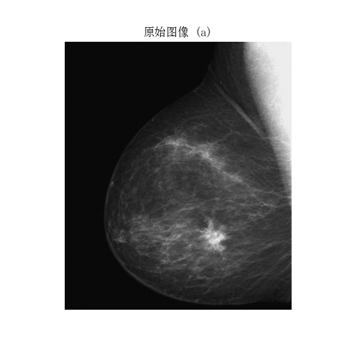
# 显示原始图像
plt.figure(figsize=(5, 5))
plt.imshow(breast_image, cmap='gray')
plt.title('原始图像 (a)')
plt.axis('off')
plt.show()

处理原理：原始图像的灰度范围通常不完全覆盖整个可能的范围（0-255），导致对比度较低。这是医学图像的常见问题，需要通过灰度变换来增强细节。

处理结果

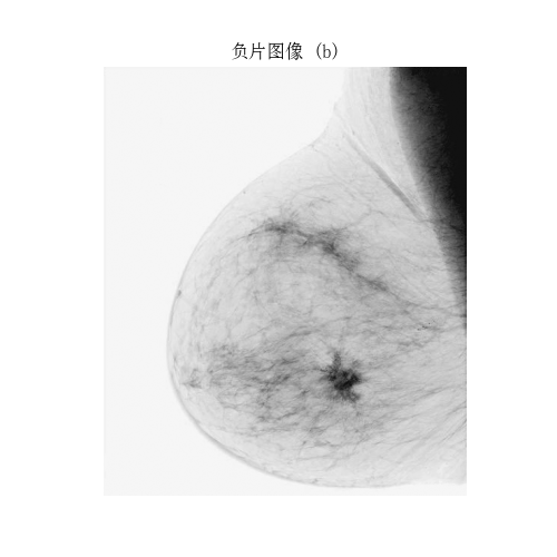
(b) 负片图像

# 负片变换 (反转变换)
negative_image = 1.0 - imadjust(breast_image, low_in=0, high_in=1)

# 转换为uint8用于显示
negative_image_uint8 = (negative_image * 255).astype(np.uint8)

# 显示结果
plt.figure(figsize=(5, 5))
plt.imshow(negative_image_uint8, cmap='gray')
plt.title('负片图像 (b)')
plt.axis('off')
plt.show()

处理原理：负片变换是灰度反转变换，公式为：
$$J=1-I$$

• 将暗部区域映射到亮部，亮部映射到暗部
• 有助于突出乳房中的异常区域（如肿瘤通常表现为亮区）
• 在医学图像处理中，负片可以增强对特定结构的观察

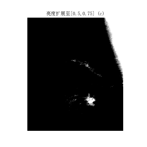
© 亮度扩展至[0.5,0.75]后的结果

# 亮度扩展至[0.5,0.75]
extended_image = imadjust(breast_image, 
                         low_in=0.5, high_in=0.75, 
                         low_out=0, high_out=1)

# 转换为uint8用于显示
extended_image_uint8 = (extended_image * 255).astype(np.uint8)

# 显示结果
plt.figure(figsize=(5, 5))
plt.imshow(extended_image_uint8, cmap='gray')
plt.title('亮度扩展至[0.5,0.75] (c)')
plt.axis('off')
plt.show()

处理原理：亮度扩展将输入图像的特定灰度范围（0.5-0.75）映射到输出范围（0-1），公式为：
$$J=\frac{I-0.5}{0.75-0.5}=\frac{I-0.5}{0.25}$$

• 输入中灰度值在[0.5, 0.75]的像素被拉伸到[0, 1]
• 低于0.5的像素映射到0（黑色）
• 高于0.75的像素映射到1（白色）
• 这种变换增强了特定亮度范围的对比度，使该范围内的细节更加清晰

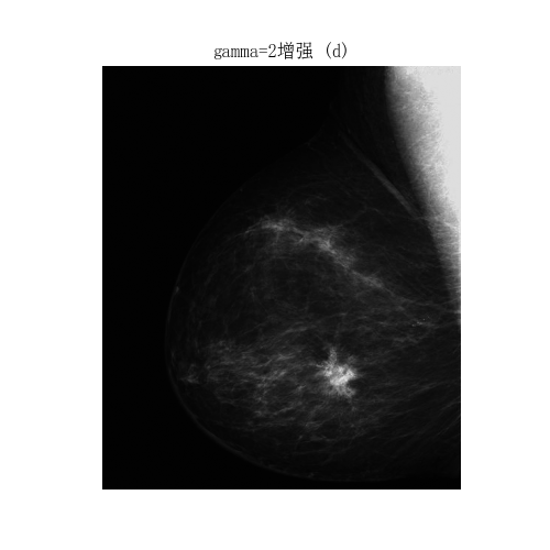
(d) 用gamma=2增强后的结果

# Gamma校正 (gamma=2)
gamma_image = imadjust(breast_image, 
                      low_in=0, high_in=1, 
                      low_out=0, high_out=1, 
                      gamma=2)

# 转换为uint8用于显示
gamma_image_uint8 = (gamma_image * 255).astype(np.uint8)

# 显示结果
plt.figure(figsize=(5, 5))
plt.imshow(gamma_image_uint8, cmap='gray')
plt.title('gamma=2增强 (d)')
plt.axis('off')
plt.show()

处理原理：Gamma校正公式为：
$$J=I^{\gamma }$$

• $\gamma =2>1$：增强暗部区域，压缩亮部区域
• 暗部细节（低灰度值）对比度增加
• 亮部细节（高灰度值）对比度减少
• 在医学图像中，这有助于突出乳房中的暗部结构（如肿瘤周围组织）

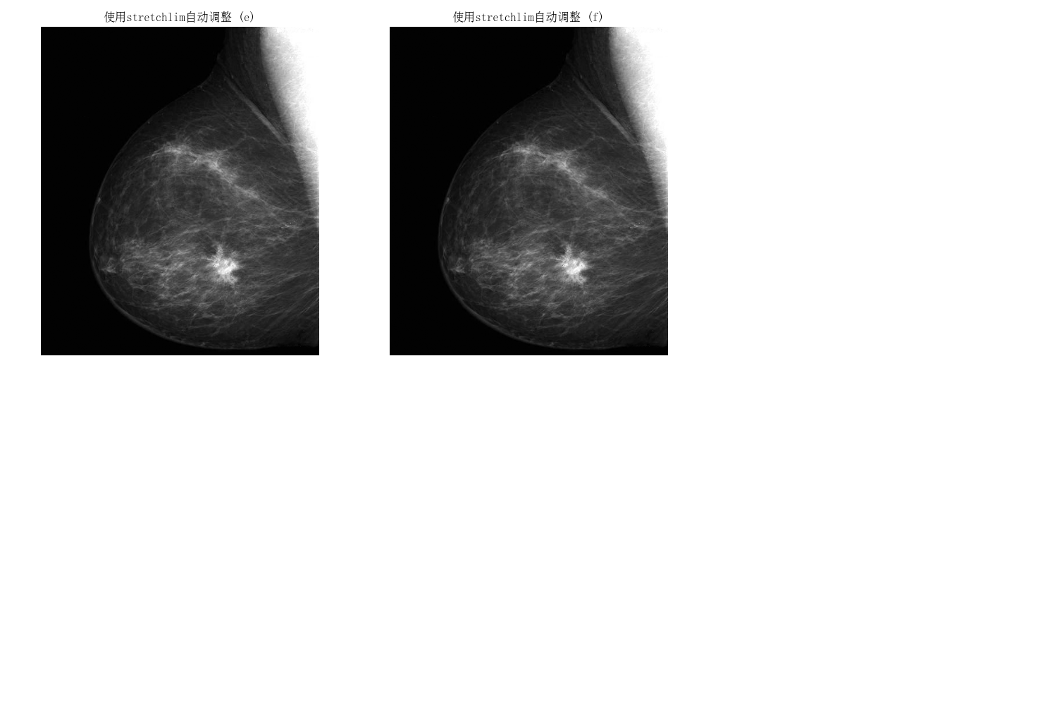
(e) 和 (f) 自动输入数据到imadjust函数（使用stretchlim）

# 计算stretchlim
stretch_limits = stretchlim(breast_image)
print("stretchlim计算的范围:", [f"{x:.4f}" for x in stretch_limits])

# (e) 使用stretchlim自动调整
stretch_image = imadjust(breast_image, 
                        low_in=stretch_limits[0], 
                        high_in=stretch_limits[1])

# (f) 使用stretchlim并指定输出范围
stretch_image_out = imadjust(breast_image, 
                           low_in=stretch_limits[0], 
                           high_in=stretch_limits[1], 
                           low_out=0, high_out=1)

# 转换为uint8用于显示
stretch_image_uint8 = (stretch_image * 255).astype(np.uint8)
stretch_image_out_uint8 = (stretch_image_out * 255).astype(np.uint8)

# 显示结果
images = [stretch_image_uint8, stretch_image_out_uint8]
titles = ['使用stretchlim自动调整 (e)', '使用stretchlim自动调整 (f)']
show_images(images, titles)

处理原理：

• stretchlim计算图像的1%和99%灰度级作为输入范围
• (e) 使用imadjust(image, stretchlim(image))：
  • 输入范围：[1%, 99%]
  • 输出范围：[0, 1]（默认）
  • 将图像中1%最暗像素映射到0，99%最亮像素映射到1
  • 中间98%的灰度线性拉伸到[0,1]
• (f) 使用imadjust(image, stretchlim(image), 0, 1)：
  • 与(e)相同，但显式指定输出范围为[0,1]
  • 实际效果与(e)相同

为什么使用stretchlim？：

• 自动适应图像内容，无需手动设置范围
• 避免图像过曝或欠曝
• 在医学图像中，能有效增强组织结构的可见性

综合分析与医学应用

灰度变换在医学图像中的重要性

在数字乳房X光成像中，灰度变换对诊断至关重要：

1. 增强对比度：使肿瘤、钙化点等异常区域更明显
2. 抑制噪声：通过调整灰度范围，减少背景噪声的影响
3. 标准化：使不同设备、不同扫描条件下的图像具有可比性

各种变换的医学应用

变换类型	适用场景	优势	注意事项
负片	观察高对比度区域	突出亮区（如钙化点）	可能使暗区难以观察
亮度扩展	放大特定亮度范围	精确增强感兴趣区域	需要先确定关键范围
Gamma校正	增强暗部细节	适合观察肿瘤周围组织	Gamma>1增强暗部，Gamma<1增强亮部
自动拉伸	通用预处理	无需手动调整，提高效率	可能过度拉伸某些区域

专业建议

1. 多方法组合：在实际诊断中，通常组合使用多种变换

   • 先用stretchlim进行自动对比度增强
   • 再用imadjust针对特定区域进行精细调整

2. 参数选择：

   • 对于乳房X光片，通常使用gamma=1.5-2.0增强暗部
   • 使用stretchlim时，可调整p1和p2（如p1=0.02, p2=0.98）避免极端值影响

3. 验证：任何图像处理都应由专业放射科医生验证，避免误导诊断

完整代码

import os
import cv2
import numpy as np
import matplotlib
matplotlib.use('Agg')  # 在导入pyplot前设置
import matplotlib.pyplot as plt
from matplotlib import gridspec

# 1. 灰度变换函数实现
def imadjust(image, low_in=0.0, high_in=1.0, low_out=0.0, high_out=1.0, gamma=1.0):
    """
    实现MATLAB的imadjust函数功能
    """
    img_float = image.astype(np.float32) / 255.0 if image.dtype == np.uint8 else image
    
    if high_in <= low_in:
        raise ValueError("high_in must be greater than low_in")
    
    normalized = (img_float - low_in) / (high_in - low_in)
    
    if gamma != 1.0:
        normalized = np.power(normalized, gamma)
    
    result = normalized * (high_out - low_out) + low_out
    result = np.clip(result, 0.0, 1.0)
    
    return result

def stretchlim(image, p1=0.01, p2=0.99):
    """
    实现MATLAB的stretchlim函数功能
    """
    img_float = image.astype(np.float32) / 255.0 if image.dtype == np.uint8 else image
    
    hist, bins = np.histogram(img_float.flatten(), bins=256, density=True)
    cdf = hist.cumsum()
    cdf = cdf / cdf[-1]
    
    low_in = bins[np.argmin(np.abs(cdf - p1))]
    high_in = bins[np.argmin(np.abs(cdf - p2))]
    
    return [low_in, high_in]
# 创建显示函数
def show_images(images, titles, figsize=(15, 10)):
    """显示多张图像"""
    plt.figure(figsize=figsize)
    gs = gridspec.GridSpec(2, 3, width_ratios=[1, 1, 1], height_ratios=[1, 1])
    
    for i, (img, title) in enumerate(zip(images, titles)):
        ax = plt.subplot(gs[i])
        if img.ndim == 2:  # 灰度图像
            plt.imshow(img, cmap='gray')
        else:  # 彩色图像
            plt.imshow(cv2.cvtColor(img, cv2.COLOR_BGR2RGB))
        plt.title(title)
        plt.axis('off')
    
    plt.tight_layout()
    plt.show()
    plt.savefig('results//chapter2-2//images.png')
# 2. 读取图像

breast_image = cv2.imread('images\\dipum_images_ch03\\Fig0303(a)(breast).tif', cv2.IMREAD_GRAYSCALE)
if breast_image is None:
    raise FileNotFoundError

os.makedirs('results//chapter2-2', exist_ok=True)
# 3. 显示原始图像
plt.figure(figsize=(5, 5))
plt.imshow(breast_image, cmap='gray')
plt.title('原始图像 (a)')
plt.axis('off')
plt.show()
plt.savefig('results//chapter2-2//原始图像 (a).png')

# 4. 负片图像
negative_image = 1.0 - imadjust(breast_image, low_in=0, high_in=1)
negative_image_uint8 = (negative_image * 255).astype(np.uint8)

plt.figure(figsize=(5, 5))
plt.imshow(negative_image_uint8, cmap='gray')
plt.title('负片图像 (b)')
plt.axis('off')
plt.show()
plt.savefig('results//chapter2-2//负片图像 (b).png')

# 5. 亮度扩展至[0.5,0.75]
extended_image = imadjust(breast_image, low_in=0.5, high_in=0.75, low_out=0, high_out=1)
extended_image_uint8 = (extended_image * 255).astype(np.uint8)

plt.figure(figsize=(5, 5))
plt.imshow(extended_image_uint8, cmap='gray')
plt.title('亮度扩展至[0.5,0.75] (c)')
plt.axis('off')
plt.show()
plt.savefig('results//chapter2-2//亮度扩展至[0.5,0.75] (c).png')

# 6. Gamma=2增强
gamma_image = imadjust(breast_image, low_in=0, high_in=1, low_out=0, high_out=1, gamma=2)
gamma_image_uint8 = (gamma_image * 255).astype(np.uint8)

plt.figure(figsize=(5, 5))
plt.imshow(gamma_image_uint8, cmap='gray')
plt.title('gamma=2增强 (d)')
plt.axis('off')
plt.show()
plt.savefig('results//chapter2-2//gamma=2增强 (d).png')

# 7. 自动调整（使用stretchlim）
stretch_limits = stretchlim(breast_image)
print("stretchlim计算的范围:", [f"{x:.4f}" for x in stretch_limits])

stretch_image = imadjust(breast_image, low_in=stretch_limits[0], high_in=stretch_limits[1])
stretch_image_out = imadjust(breast_image, low_in=stretch_limits[0], high_in=stretch_limits[1], low_out=0, high_out=1)

stretch_image_uint8 = (stretch_image * 255).astype(np.uint8)
stretch_image_out_uint8 = (stretch_image_out * 255).astype(np.uint8)

images = [stretch_image_uint8, stretch_image_out_uint8]
titles = ['使用stretchlim自动调整 (e)', '使用stretchlim自动调整 (f)']
show_images(images, titles)

总结

1. imadjust：实现灰度映射的核心函数，支持线性和非线性变换

   • 通过low_in/high_in控制输入范围
   • 通过low_out/high_out控制输出范围
   • 通过gamma实现非线性增强

2. stretchlim：自动计算图像的最佳灰度范围

   • 基于累积分布函数(CDF)
   • 默认使用1%和99%的灰度级

3. 医学应用价值：

   • 增强乳房X光片中的肿瘤和钙化点
   • 提高医生诊断准确率
   • 为计算机辅助诊断(CAD)系统提供预处理

重要提示：在实际医学应用中，所有图像处理步骤都应由专业放射科医生验证，确保处理结果不会影响诊断准确性。本教程仅用于教学目的，不应用于实际医疗诊断。

参考文献

1. Gonzalez, R. C., & Woods, R. E. (2017). Digital Image Processing (4th ed.). Pearson.
2. OpenCV Documentation: Image Processing
3. Medical Imaging: Mammography Image Enhancement
4. Gamma Correction: Understanding Gamma