算法构建了一种面向电力电缆热动力学仿真的物理信息神经网络PINN，以一维热方程为物理约束，将空间坐标与时间坐标作为输入，输出电缆温度场。通过有限差分法FDM生成带噪声的合成观测数据作为数据项，同时在域内随机采样配置点计算偏微分方程残差，并严格施加边界条件与初始条件。总损失函数由数据损失、物理残差损失、边界损失和初始损失加权构成，采用Adam优化器与阶梯学习率衰减进行训练。

算法步骤

物理问题建模

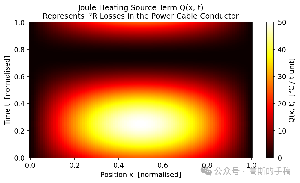
建立描述地下电缆热动态的一维热方程：∂T/∂t = α ∂²T/∂x² + Q(x,t)，其中α为热扩散系数，Q(x,t)为焦耳热源项（正弦时空分布）。确定电缆长度L=1（归一化）、总时间T=1（归一化）、环境温度20°C等物理参数。

参考数据生成（FDM求解）

采用显式FTCS有限差分格式对热方程进行数值离散，在101×1001时空网格上求解得到纯净温度场T_true，并叠加高斯噪声（σ=0.5°C）模拟真实传感器测量值T_noisy，作为PINN的数据监督项。

训练数据构建

观测数据点：从FDM网格中随机采样2000个(x,t,T_noisy)三元组。

配置点（物理残差点）：在域内均匀随机采样5000个(x,t)点，仅需坐标，用于计算PDE残差。

边界条件点：在左边界(x=0)和右边界(x=L)各采样200个时间点，目标温度恒为环境温度。

初始条件点：在t=0时刻采样200个空间点，目标温度恒为环境温度。

神经网络构建

搭建全连接神经网络，输入层2个神经元（x和t），4个隐藏层各64个神经元，激活函数为Tanh，输出层1个神经元（温度T）。采用Xavier初始化。

损失函数定义

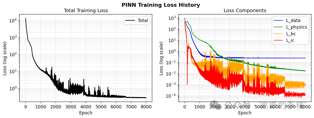
总损失 L = λ_data·MSE(T_pred, T_noisy) + λ_phys·MSE(∂T/∂t - α∂²T/∂x² - Q) + λ_bc·MSE(边界条件) + λ_ic·MSE(初始条件)。权重λ分别设为1.0、1.0、10.0、10.0。

模型训练

使用Adam优化器，初始学习率1e-3，每2000个epoch学习率减半，共训练8000个epoch。每100个epoch输出损失日志，每2000个epoch保存检查点，并保存总损失最低的模型。

评估与可视化

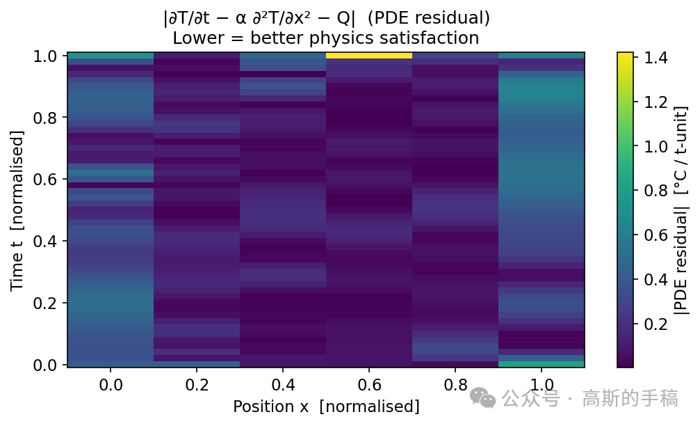
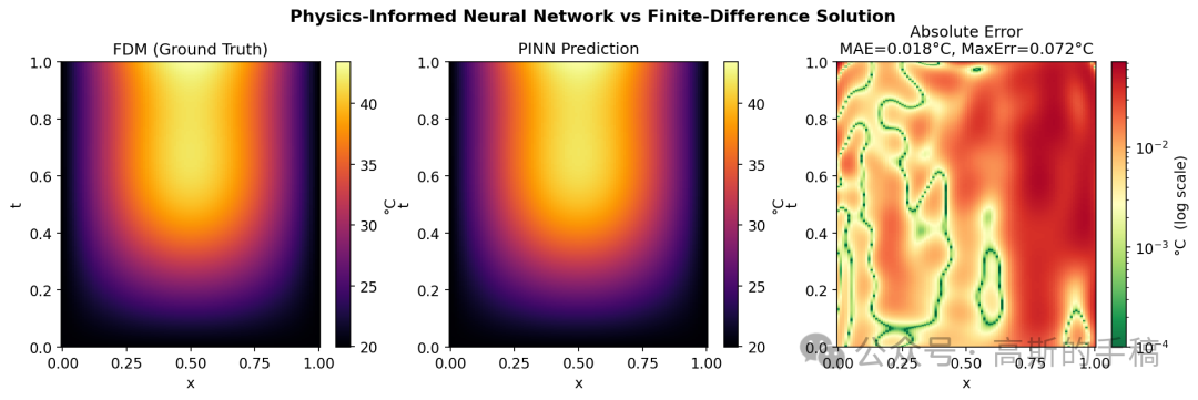
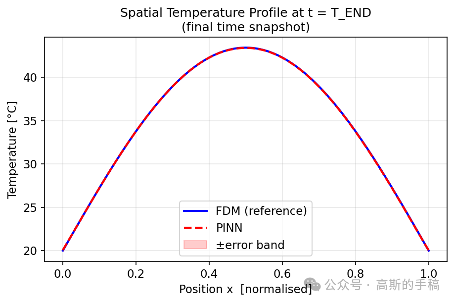
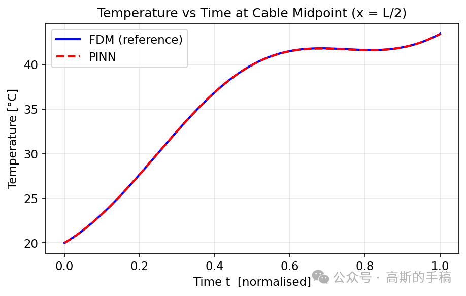
在完整FDM网格上计算PINN预测值与FDM参考值的MAE、RMSE、最大绝对误差和相对L²误差。生成温度场对比图、时空剖面图、损失曲线、PDE残差分布图等。

def heat_source_torch(x: torch.Tensor, t: torch.Tensor) -> torch.Tensor:
    """焦耳热源项 Q(x,t) 的PyTorch实现"""
    spatial_profile = torch.sin(cfg.OMEGA_X * x / cfg.L_CABLE)
    temporal_profile = 0.5 + 0.5 * torch.sin(cfg.OMEGA_T * t / cfg.T_END)
    return cfg.Q_PEAK * spatial_profile * temporal_profile

def loss_physics(model, x_col, t_col):
    """
    物理损失：计算PDE残差 f = ∂T/∂t - α ∂²T/∂x² - Q 的MSE
    自动微分求一阶和二阶导数
    """
    T_pred = model(x_col, t_col)

    # 一阶时间导数
    dT_dt = torch.autograd.grad(T_pred, t_col, 
                                grad_outputs=torch.ones_like(T_pred),
                                create_graph=True, retain_graph=True)[0]
    # 一阶空间导数
    dT_dx = torch.autograd.grad(T_pred, x_col,
                                grad_outputs=torch.ones_like(T_pred),
                                create_graph=True, retain_graph=True)[0]
    # 二阶空间导数
    d2T_dx2 = torch.autograd.grad(dT_dx, x_col,
                                  grad_outputs=torch.ones_like(dT_dx),
                                  create_graph=True)[0]

    Q = heat_source_torch(x_col, t_col)
    residual = dT_dt - cfg.ALPHA * d2T_dx2 - Q
    return torch.mean(residual ** 2)

def total_loss(model, training_data):
    """加权总损失：数据 + 物理 + 边界 + 初始"""
    L_data = torch.mean((model(training_data["x_data"], training_data["t_data"]) - training_data["T_data"]) ** 2)
    L_phys = loss_physics(model, training_data["x_col"], training_data["t_col"])

    # 边界条件损失
    x_l, t_l, T_l_target = training_data["bc_left"]
    x_r, t_r, T_r_target = training_data["bc_right"]
    L_bc = torch.mean((model(x_l, t_l) - T_l_target) ** 2) + \
           torch.mean((model(x_r, t_r) - T_r_target) ** 2)

    # 初始条件损失
    L_ic = torch.mean((model(training_data["x_ic"], training_data["t_ic"]) - training_data["T_ic"]) ** 2)

    total = cfg.LAMBDA_DATA * L_data + cfg.LAMBDA_PHYS * L_phys + \
            cfg.LAMBDA_BC * L_bc + cfg.LAMBDA_IC * L_ic
    return total, {"data": L_data.item(), "physics": L_phys.item(), 
                   "bc": L_bc.item(), "ic": L_ic.item(), "total": total.item()}


# ==================== train.py - 训练主循环 ====================
import torch.optim as optim

def train(model, training_data, n_epochs=8000):
    optimizer = optim.Adam(model.parameters(), lr=1e-3)
    scheduler = optim.lr_scheduler.StepLR(optimizer, step_size=2000, gamma=0.5)

    best_loss = float('inf')
    history = {"total": [], "data": [], "physics": [], "bc": [], "ic": []}

    for epoch in range(1, n_epochs + 1):
        optimizer.zero_grad()
        loss, comps = total_loss(model, training_data)
        loss.backward()
        torch.nn.utils.clip_grad_norm_(model.parameters(), max_norm=1.0)  # 梯度裁剪
        optimizer.step()
        scheduler.step()

        # 记录损失
        for k in history:
            history[k].append(comps[k])

        # 保存最佳模型
        if comps["total"] < best_loss:
            best_loss = comps["total"]
            torch.save(model.state_dict(), "best_model.pt")

        # 打印日志
        if epoch % 100 == 0:
            print(f"Epoch {epoch:5d} | Loss_total={comps['total']:.4f} | "
                  f"L_data={comps['data']:.4f} | L_phys={comps['physics']:.4f}")

    return history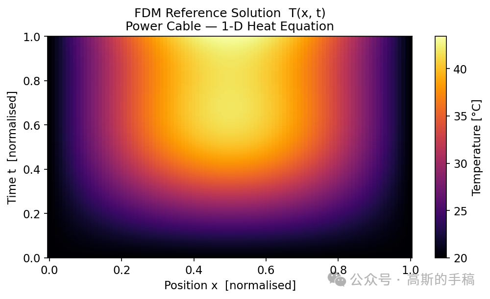

如果你对信号滤波/降噪，机器学习/深度学习，时间序列预分析/预测，设备故障诊断/缺陷检测/异常检测有疑问，或者需要论文思路上的建议，欢迎学术付费咨询

担任《MSSP》《中国电机工程学报》《宇航学报》《控制与决策》等期刊审稿专家，擅长领域：信号滤波/降噪，机器学习/深度学习，时间序列预分析/预测，设备故障诊断/缺陷检测/异常检测