@浙大疏锦行

from bayes_opt import BayesianOptimization
from xgboost import XGBClassifier
from sklearn.model_selection import cross_val_score
import numpy as np

# 定义XGBoost目标函数
def xgb_eval(n_estimators, max_depth, learning_rate, subsample, colsample_bytree, 
             reg_alpha, reg_lambda, min_child_weight):
    """
    目标函数：评估XGBoost在给定参数下的性能
    BayesianOptimization 会最大化这个函数的返回值
    
    参数说明：
    - n_estimators: 树的数量（boosting轮数）
    - max_depth: 树的最大深度
    - learning_rate: 学习率（步长）
    - subsample: 样本采样比例
    - colsample_bytree: 每棵树特征采样比例
    - reg_alpha: L1正则化系数
    - reg_lambda: L2正则化系数  
    - min_child_weight: 子节点最小权重和
    """
    # 参数处理
    n_estimators = int(n_estimators)
    max_depth = int(max_depth)
    
    # 创建XGBoost模型
    model = XGBClassifier(
        n_estimators=n_estimators,
        max_depth=max_depth,
        learning_rate=learning_rate,
        subsample=min(subsample, 0.99),  # 避免1.0
        colsample_bytree=min(colsample_bytree, 0.99),
        reg_alpha=reg_alpha,
        reg_lambda=reg_lambda,
        min_child_weight=min_child_weight,
        random_state=42,
        n_jobs=-1,
        use_label_encoder=False,
        eval_metric='logloss'
    )
    
    # 5折交叉验证
    scores = cross_val_score(model, X_train, y_train, cv=5, scoring='accuracy')
    return np.mean(scores)

# 定义XGBoost参数搜索空间
pbounds_xgb = {
    'n_estimators': (50, 1000),           # 树的数量
    'max_depth': (3, 15),                 # 树深度
    'learning_rate': (0.01, 0.3),         # 学习率
    'subsample': (0.5, 0.99),             # 样本采样
    'colsample_bytree': (0.5, 0.99),      # 特征采样
    'reg_alpha': (0, 10),                 # L1正则化
    'reg_lambda': (0, 10),                # L2正则化
    'min_child_weight': (1, 20)           # 子节点最小权重
}

# 打印参数范围
print("XGBoost参数搜索空间:")
for param, (low, high) in pbounds_xgb.items():
    range_size = high - low
    print(f"  {param:20s}: [{low:7.3f}, {high:7.3f}]  (范围: {range_size:7.3f})")

XGBoost参数搜索空间:
  n_estimators        : [ 50.000, 1000.000]  (范围: 950.000)
  max_depth           : [  3.000,  15.000]  (范围:  12.000)
  learning_rate       : [  0.010,   0.300]  (范围:   0.290)
  subsample           : [  0.500,   0.990]  (范围:   0.490)
  colsample_bytree    : [  0.500,   0.990]  (范围:   0.490)
  reg_alpha           : [  0.000,  10.000]  (范围:  10.000)
  reg_lambda          : [  0.000,  10.000]  (范围:  10.000)
  min_child_weight    : [  1.000,  20.000]  (范围:  19.000)

import time
# 创建贝叶斯优化器，优化的过程已经被这个对象封装了
optimizer = BayesianOptimization(
    f=xgb_eval, # 目标函数
    pbounds=pbounds_xgb,   # 参数搜索空间
    random_state=42,
    verbose=2  # 2: 详细信息, 1: 简要信息, 0: 不显示
)

start_time = time.time()

# 开始优化（大幅增加迭代次数以充分探索超大空间）
optimizer.maximize(
    init_points=20,  # 初始随机探索点数（增加到20以覆盖超大空间）
    n_iter=80        # 贝叶斯优化迭代次数（增加到80）
)

end_time = time.time()
print(f"优化完成！总耗时: {end_time - start_time:.2f} 秒".center(80))

# 提取所有迭代的结果
iterations = []
scores = []
for i, res in enumerate(optimizer.res): # res包含每次迭代的结果，index从0开始
    iterations.append(i + 1) # 迭代次数从1开始
    scores.append(res['target']) # 提取得分

# 计算累计最优值
best_scores = []
current_best = -np.inf # 初始化为负无穷大
for score in scores: 
    if score > current_best: # 检查当前得分是否打破历史记录
        current_best = score
    best_scores.append(current_best)

# 绘制优化轨迹
fig, (ax1, ax2) = plt.subplots(1, 2, figsize=(16, 5)) # 创建1行2列的子图

# 左图：每次迭代的得分
ax1.plot(iterations, scores, 'o-', label='每次迭代得分', alpha=0.7, markersize=6)
ax1.plot(iterations, best_scores, 'r--', label='累计最优得分', linewidth=2)
ax1.axhline(y=optimizer.max['target'], color='green', linestyle=':', 
            label=f'最终最优: {optimizer.max["target"]:.4f}') # axhline绘制水平线
ax1.set_xlabel('迭代次数', fontsize=12)
ax1.set_ylabel('准确率', fontsize=12)
ax1.set_title('贝叶斯优化收敛曲线 (超大空间100次迭代)', fontsize=14, fontweight='bold')
ax1.legend()
ax1.grid(True, alpha=0.3)

# 右图：初始探索 vs 贝叶斯优化
init_points = 20  # 更新为20
ax2.plot(iterations[:init_points], scores[:init_points], 'bo-', 
         label=f'随机探索 (前{init_points}次)', markersize=8, alpha=0.7)
ax2.plot(iterations[init_points:], scores[init_points:], 'go-', 
         label=f'贝叶斯优化 (后{len(iterations)-init_points}次)', markersize=8, alpha=0.7)
ax2.axvline(x=init_points, color='red', linestyle='--', alpha=0.5, label='探索→利用') # axvline绘制垂直线
ax2.set_xlabel('迭代次数', fontsize=12)
ax2.set_ylabel('准确率', fontsize=12)
ax2.set_title('探索阶段 vs 利用阶段', fontsize=14, fontweight='bold')
ax2.legend()
ax2.grid(True, alpha=0.3)

plt.tight_layout()
plt.show()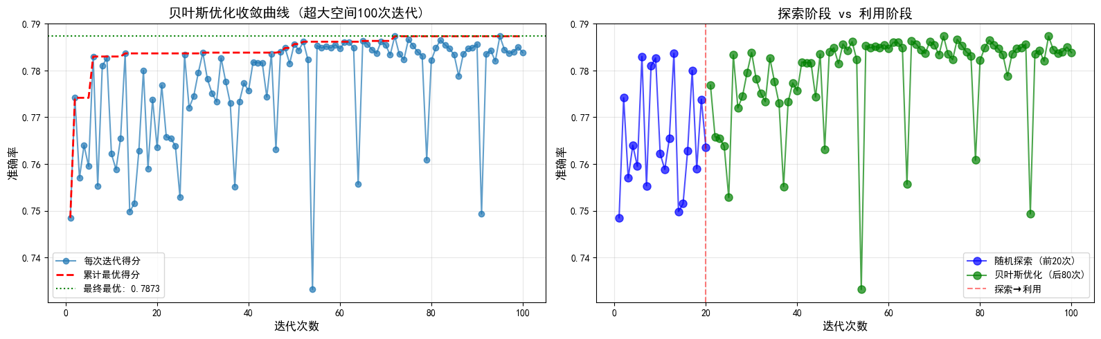

XGBoost（eXtreme Gradient Boosting）的思想可以概括为一句话

通过系统地、顺序地构建一系列“弱”的树模型，其中每一棵新树都专注于纠正前一棵树（或前一系列树）所犯的错误，最终将这些树的结果组合成一个非常强大且精确的模型。

• Extreme"表示其极致的性能优化
• "Gradient"指其使用梯度下降算法优化损失函数
• "Boosting"表示其采用提升（Boosting）集成学习方法