Day 14 Python Study
·
今日作业:
- 对信贷数据集的其他模型采取多目标优化。
- 尝试借助ai完成其他多目标问题,可借助ai生成模拟数据。@浙大疏锦行
# 先运行之前预处理好的代码
import pandas as pd
import pandas as pd    #用于数据处理和分析,可处理表格数据。
import numpy as np     #用于数值计算,提供了高效的数组操作。
import matplotlib.pyplot as plt    #用于绘制各种类型的图表
import seaborn as sns   #基于matplotlib的高级绘图库,能绘制更美观的统计图形。
import warnings
warnings.filterwarnings('ignore')  #忽略警告信息,保持输出清洁。

 # 设置中文字体(解决中文显示问题)
plt.rcParams['font.sans-serif'] = ['SimHei']  # Windows系统常用黑体字体
plt.rcParams['axes.unicode_minus'] = False    # 正常显示负号
data = pd.read_csv('E:\PyStudy\data.csv')    #读取数据

# 先筛选字符串变量
discrete_features = data.select_dtypes(include=['object']).columns.tolist()
# Home Ownership 标签编码
home_ownership_mapping = {
    'Own Home': 1,
    'Rent': 2,
    'Have Mortgage': 3,
    'Home Mortgage': 4
}
data['Home Ownership'] = data['Home Ownership'].map(home_ownership_mapping)

# Years in current job 标签编码
years_in_job_mapping = {
    '< 1 year': 1,
    '1 year': 2,
    '2 years': 3,
    '3 years': 4,
    '4 years': 5,
    '5 years': 6,
    '6 years': 7,
    '7 years': 8,
    '8 years': 9,
    '9 years': 10,
    '10+ years': 11
}
data['Years in current job'] = data['Years in current job'].map(years_in_job_mapping)

# Purpose 独热编码,记得需要将bool类型转换为数值
data = pd.get_dummies(data, columns=['Purpose'])
data2 = pd.read_csv("E:\PyStudy\data.csv") # 重新读取数据,用来做列名对比
list_final = [] # 新建一个空列表,用于存放独热编码后新增的特征名
for i in data.columns:
    if i not in data2.columns:
       list_final.append(i) # 这里打印出来的就是独热编码后的特征名
for i in list_final:
    data[i] = data[i].astype(int) # 这里的i就是独热编码后的特征名


# Term 0 - 1 映射
term_mapping = {
    'Short Term': 0,
    'Long Term': 1
}
data['Term'] = data['Term'].map(term_mapping)
data.rename(columns={'Term': 'Long Term'}, inplace=True) # 重命名列
continuous_features = data.select_dtypes(include=['int64', 'float64']).columns.tolist()  #把筛选出来的列名转换成列表

 # 连续特征用中位数补全
for feature in continuous_features:
    mode_value = data[feature].mode()[0]            #获取该列的众数。
    data[feature].fillna(mode_value, inplace=True)          #用众数填充该列的缺失值,inplace=True表示直接在原数据上修改。

# 最开始也说了 很多调参函数自带交叉验证,甚至是必选的参数,你如果想要不交叉反而实现起来会麻烦很多
# 所以这里我们还是只划分一次数据集
from sklearn.model_selection import train_test_split
X = data.drop(['Credit Default'], axis=1)  # 特征,axis=1表示按列删除
y = data['Credit Default'] # 标签
# 按照8:2划分训练集和测试集
X_train, X_test, y_train, y_test = train_test_split(X, y, test_size=0.2, random_state=42)  # 80%训练集,20%测试集


from sklearn.ensemble import RandomForestClassifier #随机森林分类器

from sklearn.metrics import accuracy_score, precision_score, recall_score, f1_score # 用于评估分类器性能的指标
from sklearn.metrics import classification_report, confusion_matrix #用于生成分类报告和混淆矩阵
import warnings #用于忽略警告信息
warnings.filterwarnings("ignore") # 忽略所有警告信息
# 评估基准模型,这里确实不需要验证集
print("--- 1. 默认参数XGboost (训练集 -> 测试集) ---")
import xgboost as xgb #XGBoost分类器
import time # 这里介绍一个新的库,time库,主要用于时间相关的操作,因为调参需要很长时间,记录下会帮助后人知道大概的时长
start_time = time.time() # 记录开始时间
# XGBoost
xgb_model = xgb.XGBClassifier(random_state=42)
xgb_model.fit(X_train, y_train)
xgb_pred = xgb_model.predict(X_test)

print("\nXGBoost 分类报告:")
print(classification_report(y_test, xgb_pred))
print("XGBoost 混淆矩阵:")
print(confusion_matrix(y_test, xgb_pred))
end_time = time.time() # 记录结束时间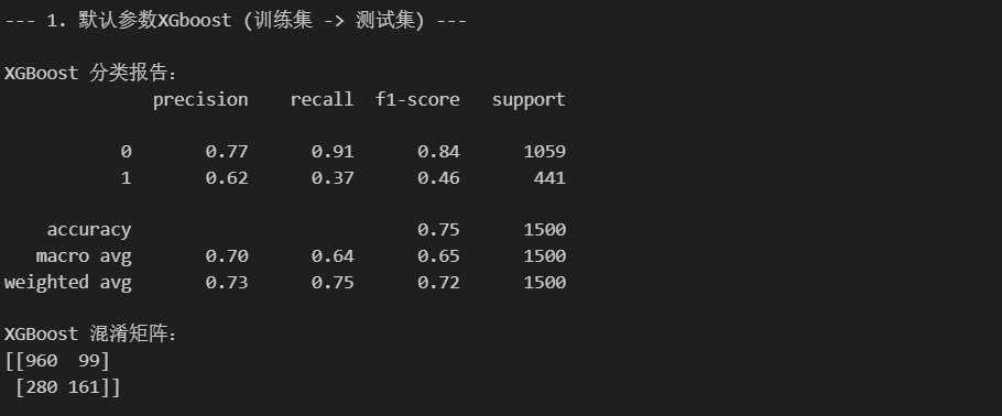
# 使用DEAP库实现NSGA-II多目标优化算法 - 修复版本
import numpy as np
from deap import base, creator, tools, algorithms
import random
from sklearn.metrics import precision_score, recall_score
from sklearn.model_selection import cross_val_score
import time
import matplotlib.pyplot as plt
import sys
import warnings
warnings.filterwarnings('ignore')

print("=== 使用DEAP库实现XGBoost多目标优化(NSGA-II算法) ===")

# 设置编码以避免字符问题
import locale
try:
    locale.setlocale(locale.LC_ALL, 'en_US.UTF-8')
except:
    pass

# 1. 定义问题
print("\n--- 步骤1: 定义多目标优化问题 ---")

# 清除之前可能存在的定义,避免冲突
if "FitnessMulti" in creator.__dict__:
    del creator.FitnessMulti
if "Individual" in creator.__dict__:
    del creator.Individual

# 创建适应度类 - 最大化精确率和召回率
creator.create("FitnessMulti", base.Fitness, weights=(1.0, 1.0))
# 创建个体类 - 包含参数列表和适应度
creator.create("Individual", list, fitness=creator.FitnessMulti)

# 2. 创建工具箱
print("--- 步骤2: 创建工具箱和定义遗传算子 ---")
toolbox = base.Toolbox()

# 参数范围定义 - 使用更合理的范围
PARAM_BOUNDS = {
    'n_estimators': (100, 500),      # 增加树的数量范围
    'max_depth': (3, 10),           # 树的最大深度
    'learning_rate': (0.01, 0.3),   # 学习率
    'subsample': (0.7, 1.0),        # 提高样本采样比例下限
    'colsample_bytree': (0.7, 1.0), # 提高特征采样比例下限
    'reg_alpha': (0, 0.5),          # 降低L1正则化范围
    'reg_lambda': (0.5, 1.0)        # 调整L2正则化范围
}

# 注册属性生成函数
toolbox.register("attr_n_estimators", random.randint, *PARAM_BOUNDS['n_estimators'])
toolbox.register("attr_max_depth", random.randint, *PARAM_BOUNDS['max_depth'])
toolbox.register("attr_learning_rate", random.uniform, *PARAM_BOUNDS['learning_rate'])
toolbox.register("attr_subsample", random.uniform, *PARAM_BOUNDS['subsample'])
toolbox.register("attr_colsample_bytree", random.uniform, *PARAM_BOUNDS['colsample_bytree'])
toolbox.register("attr_reg_alpha", random.uniform, *PARAM_BOUNDS['reg_alpha'])
toolbox.register("attr_reg_lambda", random.uniform, *PARAM_BOUNDS['reg_lambda'])

# 定义个体结构
attributes = [
    toolbox.attr_n_estimators,
    toolbox.attr_max_depth,
    toolbox.attr_learning_rate,
    toolbox.attr_subsample,
    toolbox.attr_colsample_bytree,
    toolbox.attr_reg_alpha,
    toolbox.attr_reg_lambda
]

# 注册个体和种群生成函数
toolbox.register("individual", tools.initCycle, creator.Individual, attributes, n=1)
toolbox.register("population", tools.initRepeat, list, toolbox.individual)

# 3. 定义评估函数 - 修复版本
def evaluate_xgb_individual(individual):
    """
    评估函数:计算个体的适应度(精确率和召回率)
    """
    try:
        # 解包个体参数
        (n_estimators, max_depth, learning_rate, subsample,
         colsample_bytree, reg_alpha, reg_lambda) = individual

        # 参数类型转换和边界检查
        n_estimators = max(50, min(1000, int(n_estimators)))  # 添加边界
        max_depth = max(1, min(20, int(max_depth)))
        learning_rate = max(0.001, min(1.0, learning_rate))
        subsample = max(0.1, min(1.0, subsample))
        colsample_bytree = max(0.1, min(1.0, colsample_bytree))
        reg_alpha = max(0, min(10, reg_alpha))
        reg_lambda = max(0, min(10, reg_lambda))

        # 创建XGBoost分类器 - 简化版本,避免编码问题
        model = xgb.XGBClassifier(
            n_estimators=n_estimators,
            max_depth=max_depth,
            learning_rate=learning_rate,
            subsample=subsample,
            colsample_bytree=colsample_bytree,
            reg_alpha=reg_alpha,
            reg_lambda=reg_lambda,
            random_state=42,
            use_label_encoder=False,
            eval_metric='logloss',
            n_jobs=1  # 避免并行处理问题
        )

        # 使用简单的训练测试分割而不是交叉验证,避免复杂错误
        from sklearn.model_selection import train_test_split
        X_temp, X_val, y_temp, y_val = train_test_split(
            X_train, y_train, test_size=0.3, random_state=42, stratify=y_train
        )

        # 训练模型
        model.fit(X_temp, y_temp)

        # 预测
        y_pred = model.predict(X_val)

        # 计算精确率和召回率
        precision = precision_score(y_val, y_pred, zero_division=0)
        recall = recall_score(y_val, y_pred, zero_division=0)

        # 确保返回值是浮点数
        return float(precision), float(recall)

    except Exception as e:
        # 简化错误信息,避免编码问题
        error_msg = str(e)
        if 'ascii' in error_msg:
            return 0.0, 0.0
        else:
            # 打印简化的错误信息
            print(f"Error: {error_msg[:50]}...")
            return 0.0, 0.0

# 注册评估函数
toolbox.register("evaluate", evaluate_xgb_individual)

# 辅助函数:安全计算F1-score
def safe_f1_score(precision, recall):
    """安全计算F1-score,避免除以零错误"""
    if precision + recall == 0:
        return 0.0
    return 2 * precision * recall / (precision + recall)

# 辅助函数:安全计算几何平均
def safe_geometric_mean(precision, recall):
    """安全计算几何平均,避免数学错误"""
    if precision <= 0 or recall <= 0:
        return 0.0
    return (precision * recall) ** 0.5

# 4. 定义遗传算子
print("--- 步骤3: 定义遗传算子 ---")

# 获取参数边界
low_bounds = [bounds[0] for bounds in PARAM_BOUNDS.values()]
up_bounds = [bounds[1] for bounds in PARAM_BOUNDS.values()]

# 交叉算子 - 模拟二进制交叉
toolbox.register("mate", tools.cxSimulatedBinaryBounded,
                 low=low_bounds, up=up_bounds, eta=10.0)

# 变异算子 - 多项式变异
toolbox.register("mutate", tools.mutPolynomialBounded,
                 low=low_bounds, up=up_bounds, eta=10.0, indpb=0.2)

# 选择算子 - NSGA-II选择
toolbox.register("select", tools.selNSGA2)

# 5. 运行NSGA-II算法
print("--- 步骤4: 运行NSGA-II多目标优化算法 ---")

def run_nsga2_optimization():
    """
    运行NSGA-II多目标优化算法
    """
    # 算法参数 - 使用更小的规模进行测试
    population_size = 20      # 减少种群大小
    generations = 10          # 减少进化代数
    crossover_prob = 0.8      # 交叉概率
    mutation_prob = 0.2       # 变异概率

    print(f"算法参数:")
    print(f"  - 种群大小: {population_size}")
    print(f"  - 进化代数: {generations}")
    print(f"  - 交叉概率: {crossover_prob}")
    print(f"  - 变异概率: {mutation_prob}")

    # 创建初始种群
    population = toolbox.population(n=population_size)

    # 设置统计信息
    stats = tools.Statistics(lambda ind: ind.fitness.values)
    stats.register("avg", np.mean, axis=0)
    stats.register("std", np.std, axis=0)
    stats.register("min", np.min, axis=0)
    stats.register("max", np.max, axis=0)

    # 设置帕累托前沿
    pareto_front = tools.ParetoFront()

    # 运行NSGA-II算法
    print("开始进化过程...")
    start_evolution = time.time()

    # 使用更简单的算法
    final_population, logbook = algorithms.eaSimple(
        population, toolbox,
        cxpb=crossover_prob,      # 交叉概率
        mutpb=mutation_prob,      # 变异概率
        ngen=generations,         # 进化代数
        stats=stats,              # 统计信息
        halloffame=pareto_front,  # 帕累托前沿
        verbose=True              # 显示进度
    )

    evolution_time = time.time() - start_evolution
    print(f"进化完成,耗时: {evolution_time:.2f}秒")

    return final_population, logbook, pareto_front

# 运行优化算法
print("开始多目标优化...")
start_time = time.time()

try:
    final_pop, log, pareto_front = run_nsga2_optimization()
    optimization_success = True
except Exception as e:
    print(f"优化过程失败: {e}")
    final_pop, log, pareto_front = [], None, tools.ParetoFront()
    optimization_success = False

total_time = time.time() - start_time

# 6. 分析优化结果
print("\n--- 步骤5: 分析优化结果 ---")
print(f"优化总耗时: {total_time:.2f}秒")

if optimization_success and len(pareto_front) > 0:
    print(f"找到的帕累托最优解数量: {len(pareto_front)}")

    # 过滤掉性能为0的解
    valid_solutions = [ind for ind in pareto_front if ind.fitness.values[0] > 0 or ind.fitness.values[1] > 0]

    if len(valid_solutions) > 0:
        print(f"有效帕累托最优解数量: {len(valid_solutions)}")

        # 按精确率排序显示前5个最优解
        pareto_sorted = sorted(valid_solutions, key=lambda ind: ind.fitness.values[0], reverse=True)

        print("\n帕累托前沿最优解:")
        print("-" * 80)

        for i, individual in enumerate(pareto_sorted[:5]):
            precision, recall = individual.fitness.values
            params = individual

            # 安全计算F1-score
            f1 = safe_f1_score(precision, recall)

            print(f"解 {i+1}:")
            print(f"  性能 - 精确率: {precision:.4f}, 召回率: {recall:.4f}, F1-score: {f1:.4f}")
            print(f"  参数 - n_estimators: {int(params[0])}, max_depth: {int(params[1])}")
            print(f"        learning_rate: {params[2]:.3f}, subsample: {params[3]:.3f}")
            print(f"        colsample_bytree: {params[4]:.3f}")
            print()

        # 选择最佳平衡解
        print("--- 选择最佳平衡解 ---")

        best_individual = None
        best_score = -1

        for individual in valid_solutions:
            precision, recall = individual.fitness.values
            # 使用加权评分
            score = 0.5 * precision + 0.5 * recall
            if score > best_score:
                best_score = score
                best_individual = individual

        if best_individual:
            # 解包最佳参数
            (n_estimators, max_depth, learning_rate, subsample,
             colsample_bytree, reg_alpha, reg_lambda) = best_individual

            # 参数类型转换
            n_estimators = int(n_estimators)
            max_depth = int(max_depth)

            print("选择的最佳参数:")
            print(f"  n_estimators: {n_estimators}")
            print(f"  max_depth: {max_depth}")
            print(f"  learning_rate: {learning_rate:.3f}")
            print(f"  subsample: {subsample:.3f}")
            print(f"  colsample_bytree: {colsample_bytree:.3f}")
            print(f"  reg_alpha: {reg_alpha:.3f}")
            print(f"  reg_lambda: {reg_lambda:.3f}")

            # 显示选择解的性能
            best_precision, best_recall = best_individual.fitness.values
            best_f1 = safe_f1_score(best_precision, best_recall)

            print(f"\n选择解的性能:")
            print(f"  精确率: {best_precision:.4f}")
            print(f"  召回率: {best_recall:.4f}")
            print(f"  F1-score: {best_f1:.4f}")

            # 7. 训练最终模型并评估
            print("\n--- 步骤6: 训练和评估优化后的模型 ---")

            # 使用最佳参数训练最终模型
            optimized_xgb = xgb.XGBClassifier(
                n_estimators=n_estimators,
                max_depth=max_depth,
                learning_rate=learning_rate,
                subsample=subsample,
                colsample_bytree=colsample_bytree,
                reg_alpha=reg_alpha,
                reg_lambda=reg_lambda,
                random_state=42,
                use_label_encoder=False,
                eval_metric='logloss'
            )

            optimized_xgb.fit(X_train, y_train)
            optimized_pred = optimized_xgb.predict(X_test)

            # 评估优化后的模型
            print("优化后的XGBoost模型性能:")
            print("分类报告:")
            print(classification_report(y_test, optimized_pred))
            print("混淆矩阵:")
            print(confusion_matrix(y_test, optimized_pred))

            # 性能对比
            original_precision = precision_score(y_test, xgb_pred, zero_division=0)
            original_recall = recall_score(y_test, xgb_pred, zero_division=0)
            optimized_precision = precision_score(y_test, optimized_pred, zero_division=0)
            optimized_recall = recall_score(y_test, optimized_pred, zero_division=0)

            # 安全计算F1-score
            original_f1 = safe_f1_score(original_precision, original_recall)
            optimized_f1 = safe_f1_score(optimized_precision, optimized_recall)

            print("\n--- 性能对比 ---")
            print(f"指标        | 原始模型    | 优化模型    | 提升")
            print(f"-----------|------------|------------|-------")
            print(f"精确率      | {original_precision:.4f}    | {optimized_precision:.4f}    | {optimized_precision - original_precision:+.4f}")
            print(f"召回率      | {original_recall:.4f}    | {optimized_recall:.4f}    | {optimized_recall - original_recall:+.4f}")
            print(f"F1-score   | {original_f1:.4f}    | {optimized_f1:.4f}    | {optimized_f1 - original_f1:+.4f}")

        else:
            print("未找到合适的帕累托最优解")
    else:
        print("没有找到有效的帕累托最优解(所有解的性能都为0)")
        print("可能的原因:")
        print("1. 数据预处理有问题")
        print("2. 参数范围不合适")
        print("3. 评估函数实现有误")
else:
    if not optimization_success:
        print("优化过程失败")
    else:
        print("帕累托前沿为空")

print(f"\n=== 多目标优化完成 ===")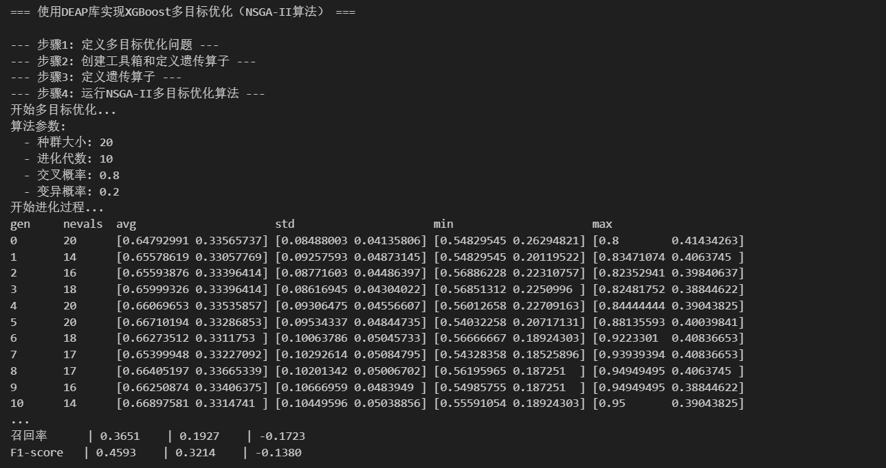
# 提取帕累托前沿并进行可视化分析
print("\n--- 帕累托前沿分析与可视化 ---")

if optimization_success and len(final_pop) > 0:
    # 1. 提取非支配解(帕累托前沿)
    print("提取帕累托前沿非支配解...")

    # 使用DEAP的工具提取非支配解
    pareto_front = tools.ParetoFront()
    pareto_front.update(final_pop)

    print(f"最终种群大小: {len(final_pop)}")
    print(f"帕累托前沿解数量: {len(pareto_front)}")

    if len(pareto_front) > 0:
        # 2. 分析帕累托前沿
        print("\n--- 帕累托前沿统计分析 ---")

        # 提取所有解的目标函数值
        all_precision = [ind.fitness.values[0] for ind in final_pop]
        all_recall = [ind.fitness.values[1] for ind in final_pop]

        # 提取帕累托解的目标函数值
        pareto_precision = [ind.fitness.values[0] for ind in pareto_front]
        pareto_recall = [ind.fitness.values[1] for ind in pareto_front]

        print(f"所有解的性能范围:")
        print(f"  精确率: [{min(all_precision):.4f}, {max(all_precision):.4f}]")
        print(f"  召回率: [{min(all_recall):.4f}, {max(all_recall):.4f}]")

        print(f"帕累托解的性能范围:")
        print(f"  精确率: [{min(pareto_precision):.4f}, {max(pareto_precision):.4f}]")
        print(f"  召回率: [{min(pareto_recall):.4f}, {max(pareto_recall):.4f}]")

        # 3. 显示帕累托前沿的多样性
        print(f"\n帕累托前沿多样性:")
        precision_range = max(pareto_precision) - min(pareto_precision)
        recall_range = max(pareto_recall) - min(pareto_recall)
        print(f"  精确率范围: {precision_range:.4f}")
        print(f"  召回率范围: {recall_range:.4f}")

        # 4. 可视化帕累托前沿
        print("\n--- 帕累托前沿可视化 ---")

        plt.figure(figsize=(15, 5))

        # 子图1: 所有解 vs 帕累托前沿
        plt.subplot(1, 3, 1)

        # 绘制所有解
        plt.scatter(all_precision, all_recall, alpha=0.6, s=30,
                   c='lightblue', label='所有解')

        # 绘制帕累托前沿
        plt.scatter(pareto_precision, pareto_recall, alpha=0.8, s=50,
                   c='red', marker='o', label='帕累托前沿')

        plt.xlabel('精确率 (Precision)')
        plt.ylabel('召回率 (Recall)')
        plt.title('NSGA-II: 所有解与帕累托前沿')
        plt.grid(True, alpha=0.3)
        plt.legend()

        # 子图2: 仅帕累托前沿
        plt.subplot(1, 3, 2)

        # 按精确率排序以便连线
        sorted_indices = np.argsort(pareto_precision)
        sorted_precision = np.array(pareto_precision)[sorted_indices]
        sorted_recall = np.array(pareto_recall)[sorted_indices]

        plt.plot(sorted_precision, sorted_recall, 'r-', alpha=0.7, linewidth=2)
        plt.scatter(pareto_precision, pareto_recall, alpha=0.8, s=60,
                   c='red', marker='o')

        plt.xlabel('精确率 (Precision)')
        plt.ylabel('召回率 (Recall)')
        plt.title('帕累托前沿')
        plt.grid(True, alpha=0.3)

        # 标记几个关键点
        if len(pareto_front) >= 3:
            # 最高精确率点
            max_precision_idx = np.argmax(pareto_precision)
            plt.annotate('最高精确率',
                        xy=(pareto_precision[max_precision_idx], pareto_recall[max_precision_idx]),
                        xytext=(10, 10), textcoords='offset points',
                        bbox=dict(boxstyle='round,pad=0.3', fc='yellow', alpha=0.7))

            # 最高召回率点
            max_recall_idx = np.argmax(pareto_recall)
            plt.annotate('最高召回率',
                        xy=(pareto_precision[max_recall_idx], pareto_recall[max_recall_idx]),
                        xytext=(10, -20), textcoords='offset points',
                        bbox=dict(boxstyle='round,pad=0.3', fc='lightgreen', alpha=0.7))

            # 平衡点(F1-score最高)
            f1_scores = [safe_f1_score(p, r) for p, r in zip(pareto_precision, pareto_recall)]
            best_f1_idx = np.argmax(f1_scores)
            plt.annotate('最佳F1-score',
                        xy=(pareto_precision[best_f1_idx], pareto_recall[best_f1_idx]),
                        xytext=(-60, 10), textcoords='offset points',
                        bbox=dict(boxstyle='round,pad=0.3', fc='orange', alpha=0.7))

        # 子图3: 解的性能分布
        plt.subplot(1, 3, 3)

        # 计算每个解的F1-score
        f1_scores_all = [safe_f1_score(p, r) for p, r in zip(all_precision, all_recall)]
        f1_scores_pareto = [safe_f1_score(p, r) for p, r in zip(pareto_precision, pareto_recall)]

        # 绘制F1-score分布
        plt.hist(f1_scores_all, bins=20, alpha=0.7, color='lightblue',
                label='所有解', density=True)
        plt.hist(f1_scores_pareto, bins=10, alpha=0.7, color='red',
                label='帕累托解', density=True)

        plt.xlabel('F1-score')
        plt.ylabel('密度')
        plt.title('F1-score分布')
        plt.legend()
        plt.grid(True, alpha=0.3)

        plt.tight_layout()
        plt.show()

        # 5. 详细分析帕累托解
        print("\n--- 帕累托解详细分析 ---")

        # 创建帕累托解的数据框以便分析
        pareto_data = []
        for i, ind in enumerate(pareto_front):
            precision, recall = ind.fitness.values
            f1 = safe_f1_score(precision, recall)
            gmean = safe_geometric_mean(precision, recall)

            pareto_data.append({
                'solution_id': i + 1,
                'precision': precision,
                'recall': recall,
                'f1_score': f1,
                'geometric_mean': gmean,
                'n_estimators': int(ind[0]),
                'max_depth': int(ind[1]),
                'learning_rate': ind[2],
                'subsample': ind[3],
                'colsample_bytree': ind[4],
                'reg_alpha': ind[5],
                'reg_lambda': ind[6]
            })

        # 转换为DataFrame
        import pandas as pd
        pareto_df = pd.DataFrame(pareto_data)

        # 显示帕累托解的关键统计信息
        print("\n帕累托解性能统计:")
        print(f"精确率 - 均值: {pareto_df['precision'].mean():.4f}, 标准差: {pareto_df['precision'].std():.4f}")
        print(f"召回率 - 均值: {pareto_df['recall'].mean():.4f}, 标准差: {pareto_df['recall'].std():.4f}")
        print(f"F1-score - 均值: {pareto_df['f1_score'].mean():.4f}, 标准差: {pareto_df['f1_score'].std():.4f}")

        # 6. 显示不同类型的解
        print("\n--- 推荐解选择 ---")

        if len(pareto_df) >= 3:
            # 精确率优先的解
            precision_focused = pareto_df.loc[pareto_df['precision'].idxmax()]
            print(f"精确率优先解:")
            print(f"  精确率: {precision_focused['precision']:.4f}, 召回率: {precision_focused['recall']:.4f}")
            print(f"  参数: n_estimators={precision_focused['n_estimators']}, max_depth={precision_focused['max_depth']}")

            # 召回率优先的解
            recall_focused = pareto_df.loc[pareto_df['recall'].idxmax()]
            print(f"召回率优先解:")
            print(f"  精确率: {recall_focused['precision']:.4f}, 召回率: {recall_focused['recall']:.4f}")
            print(f"  参数: n_estimators={recall_focused['n_estimators']}, max_depth={recall_focused['max_depth']}")

            # 平衡解 (F1-score最高)
            balanced_f1 = pareto_df.loc[pareto_df['f1_score'].idxmax()]
            print(f"平衡解 (F1-score最高):")
            print(f"  精确率: {balanced_f1['precision']:.4f}, 召回率: {balanced_f1['recall']:.4f}")
            print(f"  F1-score: {balanced_f1['f1_score']:.4f}")
            print(f"  参数: n_estimators={balanced_f1['n_estimators']}, max_depth={balanced_f1['max_depth']}")

            # 几何平均最高的解
            balanced_gmean = pareto_df.loc[pareto_df['geometric_mean'].idxmax()]
            print(f"平衡解 (几何平均最高):")
            print(f"  精确率: {balanced_gmean['precision']:.4f}, 召回率: {balanced_gmean['recall']:.4f}")
            print(f"  几何平均: {balanced_gmean['geometric_mean']:.4f}")
            print(f"  参数: n_estimators={balanced_gmean['n_estimators']}, max_depth={balanced_gmean['max_depth']}")

        # 7. 参数空间分析
        print("\n--- 参数空间分析 ---")

        # 分析重要参数的分布
        important_params = ['n_estimators', 'max_depth', 'learning_rate']

        plt.figure(figsize=(15, 4))
        for i, param in enumerate(important_params):
            plt.subplot(1, 3, i + 1)
            plt.hist(pareto_df[param], bins=15, alpha=0.7, color='skyblue', edgecolor='black')
            plt.xlabel(param)
            plt.ylabel('频数')
            plt.title(f'帕累托解 {param} 分布')
            plt.grid(True, alpha=0.3)

        plt.tight_layout()
        plt.show()

        # 8. 性能与参数关系分析
        print("\n--- 性能与参数关系 ---")

        fig, axes = plt.subplots(2, 3, figsize=(18, 10))
        axes = axes.flatten()

        param_combinations = [
            ('n_estimators', 'precision', '树数量 vs 精确率'),
            ('n_estimators', 'recall', '树数量 vs 召回率'),
            ('max_depth', 'precision', '最大深度 vs 精确率'),
            ('max_depth', 'recall', '最大深度 vs 召回率'),
            ('learning_rate', 'precision', '学习率 vs 精确率'),
            ('learning_rate', 'recall', '学习率 vs 召回率')
        ]

        for i, (x_param, y_param, title) in enumerate(param_combinations):
            if i < len(axes):
                scatter = axes[i].scatter(pareto_df[x_param], pareto_df[y_param],
                                        c=pareto_df['f1_score'], cmap='viridis',
                                        s=50, alpha=0.7)
                axes[i].set_xlabel(x_param)
                axes[i].set_ylabel(y_param)
                axes[i].set_title(title)
                axes[i].grid(True, alpha=0.3)

                # 添加颜色条
                plt.colorbar(scatter, ax=axes[i], label='F1-score')

        plt.tight_layout()
        plt.show()

        print("\n帕累托前沿分析完成!")
        print("您可以根据具体业务需求从帕累托前沿中选择合适的解:")
        print("- 如果需要高精确率:选择精确率优先的解")
        print("- 如果需要高召回率:选择召回率优先的解")
        print("- 如果需要平衡性能:选择F1-score或几何平均最高的解")

    else:
        print("未找到有效的帕累托前沿解")
else:
    print("无法进行帕累托前沿分析:优化失败或最终种群为空")

print(f"\n=== 多目标优化完整分析结束 ===")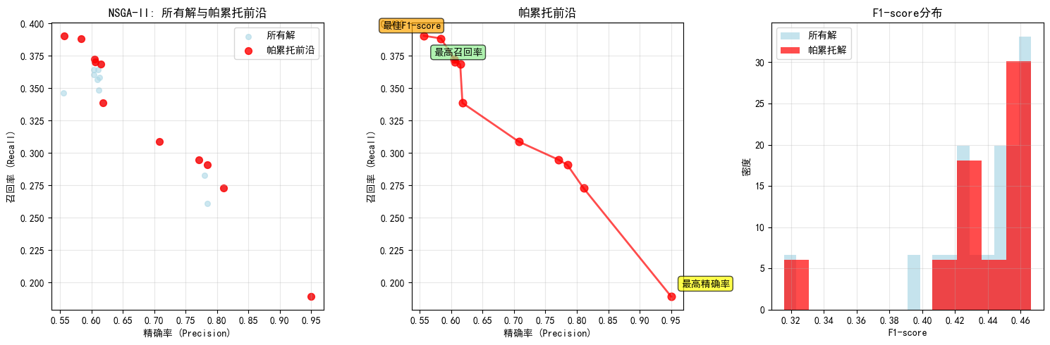

Agent 垂直技术社区,欢迎活跃、内容共建。
更多推荐
 6
6 0
0- 0


 已为社区贡献13条内容

所有评论(0)