【汽车市场数据分析与商业洞察项目（Python）——数据爬取 -  CSDN App】https://blog.csdn.net/m0_74617873/article/details/155431323?sharetype=blogdetail&shareId=155431323&sharerefer=APP&sharesource=m0_74617873&sharefrom=link

【【汽车市场数据分析与商业洞察项目（Python）】1 -  CSDN App】https://blog.csdn.net/m0_74617873/article/details/155430688?sharetype=blogdetail&shareId=155430688&sharerefer=APP&sharesource=m0_74617873&sharefrom=link

【【汽车市场数据分析与商业洞察项目（Python）】3 】 https://blog.csdn.net/m0_74617873/article/details/155430928?sharetype=blogdetail&shareId=155430928&sharerefer=APP&sharesource=m0_74617873&sharefrom=link

模块 2：销量影响因素分析（核心业务分析）

分析逻辑

1. 分析价格与销量的相关性（价格是否影响销量）
2. 对比不同能源类型的销量差异（新能源 vs 传统燃油车）
3. 分析不同车型的销量表现（SUV、轿车等哪个更受欢迎）
4. 识别头部厂商的销量优势（哪些厂商市场表现更好）

import pandas as pd
import numpy as np
import matplotlib.pyplot as plt
from datetime import datetime
from sklearn.preprocessing import MinMaxScaler

import matplotlib.pyplot as plt
import seaborn as sns
from scipy.stats import pearsonr
# 设置图形样式和中文字体
plt.rcParams['font.sans-serif'] = ['SimHei']
plt.rcParams['axes.unicode_minus'] = False

# 读取清洗后的数据
df_clean = pd.read_csv('./car_data_clean.csv')
df_clean.head()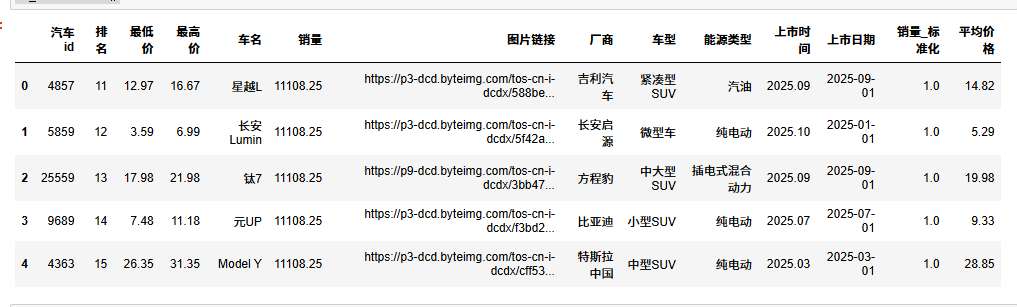

# 转换上市日期格式
df_clean['上市日期'] = pd.to_datetime(df_clean['上市日期'])

1.1  价格与销量的相关性分析

# 计算相关系数
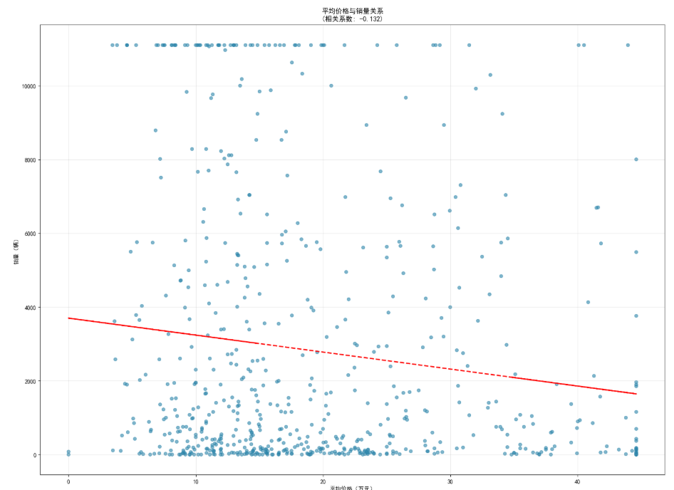
price_sales_corr, p_value = pearsonr(df_clean['平均价格'], df_clean['销量'])
print(f"平均价格与销量的皮尔逊相关系数: {round(price_sales_corr, 3)}")
print(f"相关性显著性p值: {round(p_value, 5)}")

平均价格与销量的皮尔逊相关系数: -0.132
相关性显著性p值: 0.00066

# 判断相关性强度
if abs(price_sales_corr) < 0.3:
    corr_strength = "弱相关"
elif abs(price_sales_corr) < 0.7:
    corr_strength = "中等相关"
else:
    corr_strength = "强相关"

if p_value < 0.05:
    significance = "统计显著"
else:
    significance = "统计不显著"

print(f"结论: 平均价格与销量呈{corr_strength}，{significance}")

结论: 平均价格与销量呈弱相关，统计显著

# 绘制价格-销量散点图
plt.figure(figsize=(16, 12))
plt.subplot()
plt.scatter(df_clean['平均价格'], df_clean['销量'], alpha=0.6, color='#2E86AB', s=30)
# 添加趋势线
z = np.polyfit(df_clean['平均价格'], df_clean['销量'], 1)
p = np.poly1d(z)
plt.plot(df_clean['平均价格'], p(df_clean['平均价格']), "r--", linewidth=2)
plt.title(f'平均价格与销量关系\n(相关系数: {round(price_sales_corr, 3)})', fontsize=12, fontweight='bold')
plt.xlabel('平均价格（万元）', fontsize=10)
plt.ylabel('销量（辆）', fontsize=10)
plt.grid(True, alpha=0.3)
plt.tight_layout()
plt.savefig('./价格-销量散点图.png', dpi=300, bbox_inches='tight')
plt.show()

不同能源类型的销量对比

# 计算各能源类型的销量统计
energy_sales = df_clean.groupby('能源类型')['销量'].agg(['count', 'mean', 'sum']).round(2)
energy_sales.columns = ['车型数量', '平均销量', '总销量']
energy_sales = energy_sales.sort_values('总销量', ascending=False)
print("各能源类型销量统计:")
energy_sales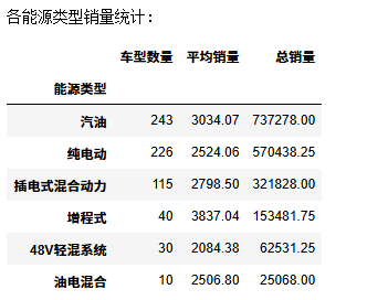

# 计算各能源类型的市场份额（按总销量）
energy_sales['市场份额(%)'] = round((energy_sales['总销量'] / energy_sales['总销量'].sum()) * 100, 2)
print(f"\n各能源类型市场份额:")
for energy, share in energy_sales['市场份额(%)'].items():
    print(f"{energy}: {share}%")

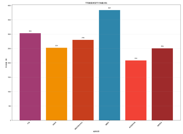
各能源类型市场份额:
汽油: 39.41%
纯电动: 30.49%
插电式混合动力: 17.2%
增程式: 8.2%
48V轻混系统: 3.34%
油电混合: 1.34%

# 绘制能源类型销量对比条形图
plt.figure(figsize=(16, 12))
plt.subplot()
colors = ['#A23B72', '#F18F01', '#C73E1D', '#2E86AB', '#F24236', '#9E2A2B']
bars = plt.bar(energy_sales.index, energy_sales['平均销量'], color=colors[:len(energy_sales)])
plt.title('不同能源类型平均销量对比', fontsize=12, fontweight='bold')
plt.xlabel('能源类型', fontsize=10)
plt.ylabel('平均销量（辆）', fontsize=10)
plt.xticks(rotation=45, ha='right')
# 在柱子上添加数值标签
for bar in bars:
    height = bar.get_height()
    plt.text(bar.get_x() + bar.get_width()/2., height + 50,
             f'{int(height)}', ha='center', va='bottom', fontsize=9)
plt.grid(True, alpha=0.3, axis='y')
plt.tight_layout()
plt.savefig('./能源类型销量对比条形图.png', dpi=300, bbox_inches='tight')
plt.show()

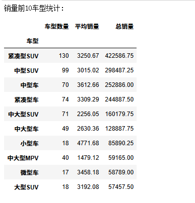
热门车型销量分析（取销量前10的车型）

# 计算各车型的销量统计
model_sales = df_clean.groupby('车型')['销量'].agg(['count', 'mean', 'sum']).round(2)
model_sales.columns = ['车型数量', '平均销量', '总销量']
top10_models = model_sales.sort_values('总销量', ascending=False).head(10)
print("销量前10车型统计:")
top10_models

# 绘制热门车型销量条形图
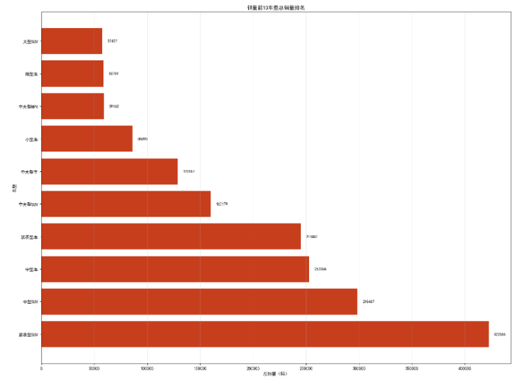
plt.figure(figsize=(16, 12))
plt.subplot()
bars = plt.barh(range(len(top10_models)), top10_models['总销量'], color='#C73E1D')
plt.yticks(range(len(top10_models)), top10_models.index)
plt.title('销量前10车型总销量排名', fontsize=12, fontweight='bold')
plt.xlabel('总销量（辆）', fontsize=10)
plt.ylabel('车型', fontsize=10)
# 在柱子上添加数值标签
for i, bar in enumerate(bars):
    width = bar.get_width()
    plt.text(width + 5000, bar.get_y() + bar.get_height()/2.,
             f'{int(width)}', ha='left', va='center', fontsize=9)
plt.grid(True, alpha=0.3, axis='x')
plt.tight_layout()
plt.savefig('./销量前10车型总销量排名.png', dpi=300, bbox_inches='tight')
plt.show()

头部厂商销量分析（取销量前10的厂商）

# 计算各厂商的销量统计
brand_sales = df_clean.groupby('厂商')['销量'].agg(['count', 'mean', 'sum']).round(2)
brand_sales.columns = ['车型数量', '平均销量', '总销量']
top10_brands = brand_sales.sort_values('总销量', ascending=False).head(10)
print("销量前10厂商统计:")
top10_brands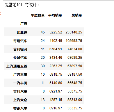

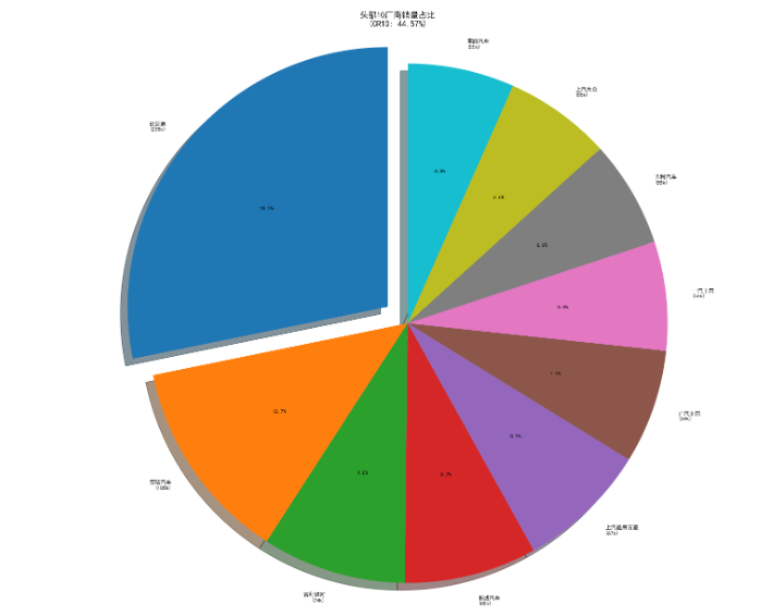
# 计算头部厂商的市场集中度（CR10）
cr10 = round((top10_brands['总销量'].sum() / df_clean['销量'].sum()) * 100, 2)
print(f"\n头部10厂商市场集中度（CR10）: {cr10}%")

头部10厂商市场集中度（CR10）: 44.57%

# 绘制头部厂商销量饼图
plt.figure(figsize=(16, 12))
plt.subplot()
# 准备饼图数据
sizes = top10_brands['总销量'].values
labels = [f'{brand}\n({int(sales/1000)}k)' for brand, sales in zip(top10_brands.index, sizes)]
# 突出显示第一名
explode = [0.1 if i == 0 else 0 for i in range(len(sizes))]

plt.pie(sizes, explode=explode, labels=labels, autopct='%1.1f%%',
        shadow=True, startangle=90, textprops={'fontsize': 8})
plt.axis('equal')
plt.title(f'头部10厂商销量占比\n(CR10: {cr10}%)', fontsize=12, fontweight='bold')
plt.tight_layout()
plt.savefig('./头部10厂商销量占比.png', dpi=300, bbox_inches='tight')
plt.show()

销量影响因素分析报告）：
1. 价格影响：平均价格与销量呈弱相关（相关系数-0.132），统计显著，说明价格是影响销量的重要因素
2. 能源类型：汽油车型表现最佳，市场份额39.41%，新能源汽车（纯电动+插电混动）合计市场份额达47.69%
3. 车型偏好：紧凑型SUV是最受欢迎车型，总销量达422586辆，SUV类车型整体表现优于其他类型
4. 厂商竞争：比亚迪占据市场领先地位，头部10厂商市场集中度（CR10）达44.57%，市场呈现寡头竞争格局
5. 业务建议：建议重点关注汽油+紧凑型SUV的产品组合，同时关注头部厂商的竞争策略