from sklearn.cross_decomposition import PLSRegression
from sklearn.model_selection import cross_val_predict
from sklearn.metrics import mean_squared_error, r2_score
from sklearn.datasets import make_regression
import numpy as np
import matplotlib.pyplot as plt

X, y = make_regression(n_samples=5000, n_features=200, noise=1, random_state=42)

def pls_evaluate_num_comp(X, y, num_comp):
    pls = PLSRegression(n_components=num_comp)
    y_cv = cross_val_predict(pls, X, y, cv=5)
    mse = mean_squared_error(y_cv, y)
    r2 = r2_score(y_cv, y)
    rpd = y.std()/np.sqrt(mse)
    return (y_cv, mse, r2, rpd)

def pls_evaluate_num_comps(X, y, num_comps):
    mses = []
    r2s = []
    rpds = []
    for num_comp in num_comps:
        _, mse, r2, rpd = pls_evaluate_num_comp(X, y, num_comp)
        mses.append(mse)
        r2s.append(r2)
        rpds.append(rpd)
    return (mses, r2s, rpds)

def plot_metric(num_comps, scores, objective, yLabel='y'):
    with plt.style.context('ggplot'):
        plt.plot(num_comps, scores, '-o', color='blue')
        idx = np.argmin(scores) if objective == 'min' else np.argmax(scores)
        plt.plot(num_comps[idx], scores[idx], 'P', color='red', ms=10)
        plt.xlabel("Number of components")
        plt.ylabel(yLabel)
    plt.show()
    return (num_comps[idx], scores[idx])

def pls_evaluate_plot_num_comps(X, y, num_comps):
    mses, r2s, rpds = pls_evaluate_num_comps(X, y, num_comps)
    # Plot mses
    num_comp, mse = plot_metric(num_comps, mses, 'min', 'MSE')
    print(f'The best mse is {mse} with {num_comp} PLS components')
    # Plot r2s
    num_comp, r2  = plot_metric(num_comps, r2s, 'max', 'R2')
    print(f'The best r2 is {r2} with {num_comp} PLS components')
    # Plot rpds
    num_comp, rpd = plot_metric(num_comps, rpds, 'max', 'RPD')
    print(f'The best RPD is {rpd} with {num_comp} PLS components')

num_comps = np.arange(1, 16)
pls_evaluate_plot_num_comps(X, y, num_comps)

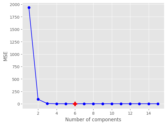
The best mse is 1.0572918939776803 with 6 PLS components.

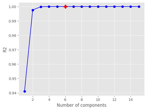
The best r2 is 0.999971948294708 with 6 PLS components.

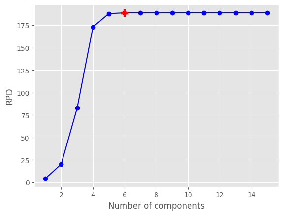
The best RPD is 188.8100894546761 with 6 PLS components.